10_Introduction to Artificial Neural Networks w Keras_3_FashionMNIST_pydot_sparse_shift(0.)_plt_imgs

10_Introduction to Artificial Neural Networks with Keras_HuberLoss_astype_dtype_DNN_MLP_G.gv.pdf_mnist

https://blog.csdn.net/Linli522362242/article/details/106433059

10_Introduction to Artificial Neural Networks with Keras_2_tensorflow2.1_Anaconda3-2019.10(python3.7.4)
https://blog.csdn.net/Linli522362242/article/details/106537459

Building an Image Classifier Using the Sequential API

     First, we need to load a dataset. In this chapter we will tackle Fashion MNIST, which is a drop-in replacement of MNIST (introduced in Cp3 https://blog.csdn.net/Linli522362242/article/details/103786116). It has the exact same format as MNIST (70,000 grayscale images of 28 × 28 pixels each, with 10 classes), but the images represent fashion items rather than handwritten digits, so each class is more diverse, and the problem turns out to be significantly more challenging than MNIST. For example, a simple linear model reaches about 92% accuracy on MNIST, but only about 83% on Fashion MNIST.

Using Keras to load the dataset

     Keras provides some utility functions to fetch and load common datasets, including MNIST, Fashion MNIST, and the California housing dataset we used in Chapter 2.
     Let's start by loading the fashion MNIST dataset. Keras has a number of functions to load popular datasets in keras.datasets. The dataset is already split for you between a training set and a test set, but it can be useful to split the training set further to have a validation set:

fashion_mnist = keras.datasets.fashion_mnist
(X_train_full, y_train_full), (X_test, y_test) = fashion_mnist.load_data()

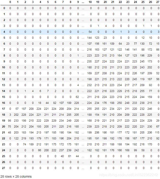
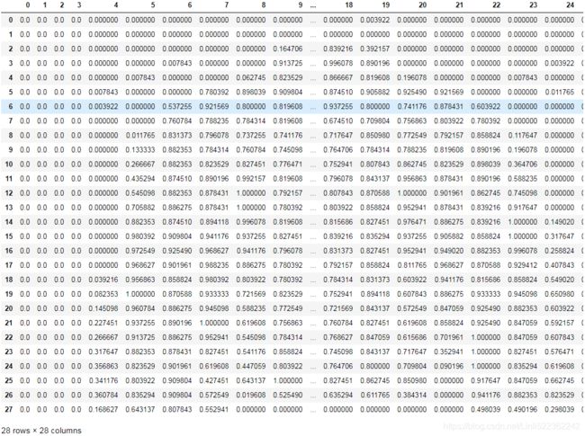
     When loading MNIST or Fashion MNIST using Keras rather than Scikit-Learn, one important difference is that every image is represented as a 28 × 28 array rather than a 1D array of size 784. Moreover, the pixel intensities are represented as integers (from 0 to 255) rather than floats (from 0.0 to 255.0). Let’s take a look at the shape and data type of the training set:

X_train_full.shape

X_train_full.dtype

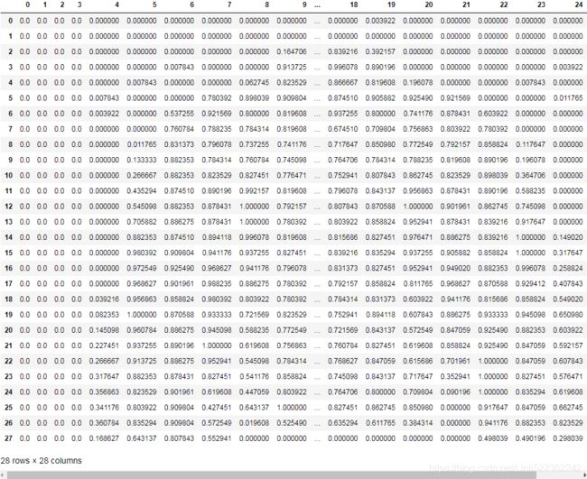
     Note that the dataset is already split into a training set and a test set, but there is no validation set, so we’ll create one now. Additionally, since we are going to train the neural network using Gradient Descent, we must scale the input features. For simplicity, we’ll scale the pixel intensities down to the 0–1 range by dividing them by 255.0 (this also converts them to floats):

import pandas as pd
pd.DataFrame(X_train_full[0])

# scale the pixel intensities down to the 0–1 range by dividing them by 255.0 (this also converts them to floats)
X_valid, X_train = X_train_full[:5000]/255. , X_train_full[5000:]/255.
y_valid, y_train = y_train_full[:5000], y_train_full[5000:]
X_test = X_test/255.   # X_test = X_test.astype('float32')/255

pd.DataFrame(X_train[0])

plt.imshow(X_train_full[5000])
plt.axis("off")
plt.show()

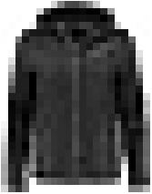
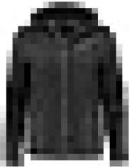
You can plot an image using Matplotlib's imshow() function, with a 'binary' color map:

import matplotlib.pyplot as plt
plt.imshow(X_train[0], cmap="binary")
plt.axis("off")
plt.show()

                                                                      

https://www.tensorflow.org/api_docs/python/tf/keras/datasets/fashion_mnist/load_data

The labels are the class IDs (represented as uint8), from 0 to 9:

y_train

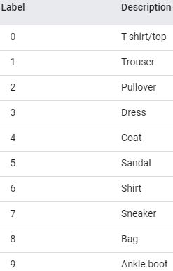
     With MNIST, when the label is equal to 5, it means that the image represents the handwritten digit 5. Easy. For Fashion MNIST, however, we need the list of class names to know what we are dealing with:
     Here are the corresponding class names:

class_names = ["T-shirt/top", "Trouser", "Pullover", "Dress", "Coat","Sandal", "Shirt", 
               "Sneaker", "Bag", "Ankle boot"]

For example, the first image in the training set represents a coat:

class_names[y_train[0]]

The validation set contains 5,000 images, and the test set contains 10,000 images:

X_valid.shape

X_test.shape

        

Let's take a look at a sample of the images in the dataset:

n_rows = 4
n_cols = 10

plt.figure( figsize=(n_cols*1.2, n_rows*1.2) ) # 0.2: for the extra space 

for row in range(n_rows):
    for col in range(n_cols):
        index = n_cols * row + col
        plt.subplot( n_rows, n_cols, index+1 ) # the subplot's index start 1
        plt.imshow(X_train[index], cmap="binary", interpolation="nearest" )
        plt.axis("off") #remove the axis
        plt.title(class_names[y_train[index]], fontsize=12)
        
plt.subplots_adjust(wspace=0.2, hspace=0.5)
plt.show()

Creating the model using the Sequential API

     Now let’s build the neural network! Here is a classification MLP with two hidden layers:

The ReLU function (introduced in https://blog.csdn.net/Linli522362242/article/details/106325257) ReLU (z) = max (0, z)

in practice it works very well and has the advantage of being fast to compute. 

Equation 4-19. Softmax score for class k   https://blog.csdn.net/Linli522362242/article/details/104124771

Equation 4-20. Softmax function 
Equation 4-21. Softmax Regression classifier prediction 

Layers, which are combined into a network (or model)

n_hidden1 = 300
n_hidden2 = 100
n_outputs = 10

model = keras.models.Sequential()
# It is a Flatten layer whose role is to convert each input image into a 1D array
model.add( keras.layers.Flatten( input_shape=[28,28] ) )

#model.add( keras.layers.Dense(512, activation="relu", input_shape=(28*28,))) if not model.add( keras.layers.Flatten( input_shape=[28,28] ) )

model.add( keras.layers.Dense(n_hidden1, activation="relu" ) ) # hidden1 layer
model.add( keras.layers.Dense(n_hidden2, activation="relu" ) ) # hidden2 layer
model.add( keras.layers.Dense(n_outputs, activation="softmax" ) ) # output layer

Let’s go through this code line by line:

• The first line creates a Sequential model. This is the simplest kind of Keras model for neural networks that are just composed of a single stack of layers connected sequentially. This is called the Sequential API.
   
• Next, we build the first layer and add it to the model. It is a Flatten layer whose role is to convert each input image into a 1D array: if it receives input data X, it computes X.reshape(-1, 1). This layer does not have any parameters; it is just there to do some simple preprocessing. Since it is the first layer in the model, you should specify the input_shape, which doesn’t include the batch size, only the shape of the instances. Alternatively, you could add a keras.layers.InputLayer as the first layer, setting input_shape=[28,28].
   
• Next we add a Dense hidden layer with 300 neurons. It will use the ReLU activation function. Each Dense layer manages its own weight matrix, containing all the connection weights between the neurons and their inputs. It also manages a vector of bias terms (one per neuron). When it receives some input data, it computes Equation 10-2. 
  
  
• Then we add a second Dense hidden layer with 100 neurons, also using the ReLU activation function.
   
• Finally, we add a Dense output layer with 10 neurons (one per class(0~9)), using the softmax activation function (because the classes are exclusive).

###########################
     Specifying activation="relu" is equivalent to specifying activation=keras.activations.relu. Other activation functions are
available in the keras.activations package, we will use many of them in this book. See https://keras.io/activations/ for the full list.
###########################

import numpy as np

keras.backend.clear_session()
np.random.seed(42)
tf.random.set_seed(42)

     Instead of adding the layers one by one as we just did, you can pass a list of layers when creating the Sequential model:

model = keras.models.Sequential([
    ## It is a Flatten layer whose role is to convert each input image into a 1D array
    keras.layers.Flatten( input_shape=[28,28] ),
    keras.layers.Dense( 300, activation="relu" ),          # hidden1 layer
    keras.layers.Dense( 100, activation="relu" ),          # hidden2 layer
    keras.layers.Dense( n_outputs, activation="softmax" )  # output layer
])

######################################################
Using Code Examples from keras.io

     Code examples documented on keras.io will work fine with tf.keras, but you need to change the imports.
For example, consider this keras.io code:

from keras.layers import Dense

output_layer = Dense(10)

You must change the imports like this:

from tensorflow.keras.layers import Dense

output_layer = Dense(10)

Or simply use full paths, if you prefer:

from tensorflow import keras

output_layer = keras.layers.Dense(10)

This approach is more verbose冗长的, but I use it in this book so you can easily see which packages to use, and to avoid confusion between standard classes and custom classes. In production code, I prefer the previous approach. Many people also use from tensorflow.keras import layers followed by layers.Dense(10).
######################################################

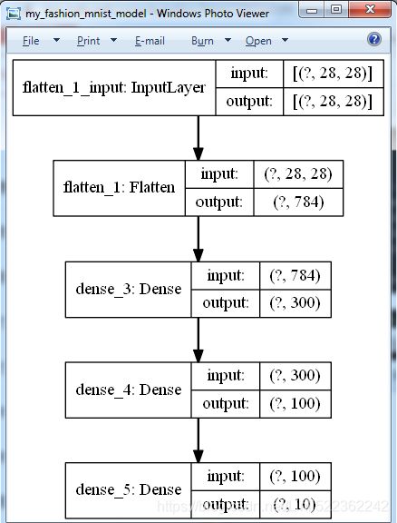
     The model’s summary() method displays all the model’s layers,###You can use keras.utils.plot_model() to generate an image of your model.### including each layer’s name (which is automatically generated unless you set it when creating the layer), its output shape (None means the batch size can be anything), and its number of parameters. The summary ends with the total number of parameters, including trainable and non-trainable parameters. Here we only have trainable parameters (we will see examples of non-trainable parameters in Chapter 11):

model.summary()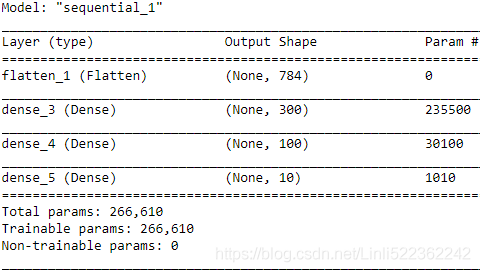

 ==> 
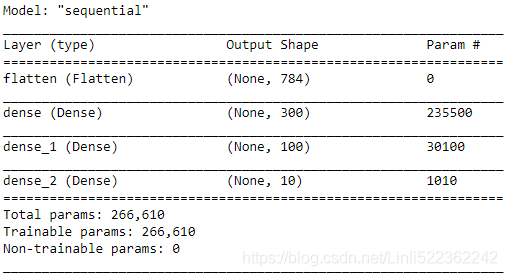
     Note that Dense layers often have a lot of parameters. For example, the first hidden layer has 784 × 300 connection weights, plus 300 bias terms, which adds up to 235,500 parameters! This gives the model quite a lot of flexibility to fit the training data, but it also means that the model runs the risk of overfitting, especially when you do not have a lot of training data. We will come back to this later.

You can easily get a model’s list of layers, to fetch a layer by its index, or you can fetch it by name:

model.layers

hidden1 = model.layers[1] # hidden1 layer
hidden1.name

model.get_layer("dense") is hidden1

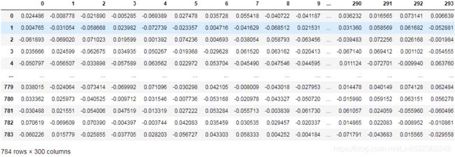
     All the parameters of a layer can be accessed using its get_weights() and set_weights() methods. For a Dense layer, this includes both the connection weights and the bias terms:

weights, biases = hidden1.get_weights()
pd.DataFrame(weights)

biases

biases.shape

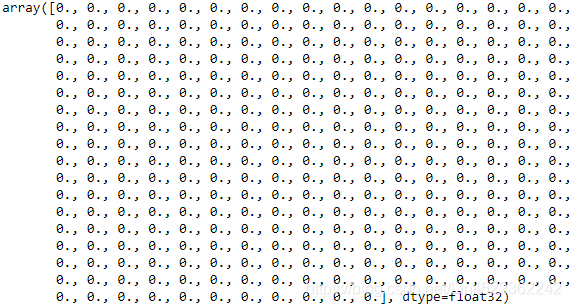
     Notice that the Dense layer initialized the connection weights randomly (which is needed to break symmetry, as we discussed earlier), and the biases were initialized to zeros, which is fine. If you ever want to use a different initialization method, you can set kernel_initializer (kernel is another name for the matrix of connection weights) or bias_initializer when creating the layer. We will discuss initializers further in Chapter 11, but if you want the full list, see https://keras.io/initializers/.

##############################################
     The shape of the weight matrix depends on the number of inputs. This is why it is recommended to specify the input_shape when creating the first layer in a Sequential model. However, if you do not specify the input shape, it’s OK: Keras will simply wait until it knows the input shape before it actually builds the model. This will happen either when you feed it actual data (e.g., during training), or when you call its build() method. Until the model is really built, the layers will not have any weights, and you will not be able to do certain things (such as print the model summary or save the model). So, if you know the input shape when creating the model, it is best to specify it.
##############################################

keras.utils.plot_model(model, "my_fashion_mnist_model.png", show_shapes=True)

 Failed to import pydot. You must install pydot and graphviz for `pydotprint` to work.

since I have installed graphviz and pydot follow the steps on https://blog.csdn.net/Linli522362242/article/details/106537459

 I think I should not use jupyter notebook for this code

So I use tensorflow Spyder before I restart my system

from tensorflow import keras

n_hidden1 = 300
n_hidden2 = 100
n_outputs = 10

model = keras.models.Sequential([
    ## It is a Flatten layer whose role is to convert each input image into a 1D array
    keras.layers.Flatten( input_shape=[28,28] ),
    keras.layers.Dense( 300, activation="relu" ),          # hidden1 layer
    keras.layers.Dense( 100, activation="relu" ),          # hidden2 layer
    keras.layers.Dense( n_outputs, activation="softmax" )  # output layer
])
keras.utils.plot_model(model, to_file="my_fashion_mnist_model.png", show_shapes=True)

 
    

After I restart my system:

keras.utils.plot_model(model, to_file="my_fashion_mnist_model.png", show_shapes=True)

 

     So I think the previous error "Failed to import pydot. You must install pydot and graphviz for `pydotprint` to work." after I installed graphviz and pydot was caused by another program which used the graphviz and the sytem had not completely closed it.

Compiling the model

     After a model is created, you must call its compile() method to specify the loss function and the optimizer to use. Optionally, you can specify a list of extra metrics to compute during training and evaluation:

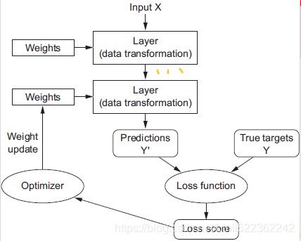
• A loss function—How the network will be able to measure its performance on the training data, and thus how it will be able to steer操纵 itself in the right direction.  The loss function, which defines the feedback signal used for learning. Here, The quantity(loss="sparse_categorical_crossentropy") that will be minimized during training. It represents a measure of success for the task at hand.  Choosing the right objective function for the right problem is extremely important.
  
  For instance, you’ll use binary crossentropy for a two-class classification problem,
  categorical crossentropy for a many-class classification problem,
  mean squared error for a regression problem,
  connectionist temporal classification (CTC) for a sequence-learning problem, and so on.
  Only when you’re working on truly new research problems will you have to develop your own objective functions. In the next few chapters, we’ll detail explicitly which loss functions to choose for a wide range of
  common tasks.
   
• An optimizer—The mechanism through which the network(model) will update itself based on the data it sees and its loss function.
                            It implements a specific variant of stochastic gradient descent (SGD).
   
• Metrics to monitor during training and testing—Here, we’ll only care about accuracy score(the fraction of the images that were correctly classified).

model.compile( loss="sparse_categorical_crossentropy", # loss=keras.losses.sparse_categorical_crossentropy
              optimizer="sgd",                         # optimizer=keras.optimizers.SGD()
              metrics=["accuracy"])                    #metrics=[keras.metrics.sparse_categorical_accuracy]

################################
Note

        This is equivalent to:

model.compile(loss=keras.losses.sparse_categorical_crossentropy,
              optimizer=keras.optimizers.SGD(),
              metrics=[keras.metrics.sparse_categorical_accuracy])

     We will use many other losses, optimizers, and metrics in this book; for the full lists, see https://keras.io/losses, https://keras.io/optimizers, and https://keras.io/metrics.
################################

     This code requires some explanation. First, we use the "sparse_categorical_cross entropy" loss because we have sparse labels (i.e., for each instance, there only just has one target class index, from 0 to 9 in this case), and the classes are exclusive (such as the target class index 3, which is used to represented 'Dress'). If instead we had one target probability per class for each instance (such as one-hot vectors, e.g. [0., 0., 0., 1., 0., 0., 0., 0., 0., 0.] to represent class 3 ###keras.utils.to_categorical( y_train )##), then we would need to use the "categorical_crossentropy" loss instead. If we were doing binary classification (with one or more binary labels), then we would use the "sigmoid" (i.e., logistic  
https://blog.csdn.net/Linli522362242/article/details/93698989) activation function in the output layer instead of the "softmax" activation function, and we would use the "binary_crossentropy" loss(https://blog.csdn.net/Linli522362242/article/details/104124771).

a sparse matrix only stores the location of the nonzero elements ##cp2## https://blog.csdn.net/Linli522362242/article/details/103387527

 ###a sparse matrix

housing_cat_1hot.toarray()       #'<1H OCEAN', 'NEAR OCEAN', 'INLAND', 'NEAR BAY', 'ISLAND'  #if exists columname

###every element in the 2D array is an one-hot vector
OR 

y_train

array([5, 0, 4, ..., 5, 6, 8], dtype=uint8)

y_train = keras.utils.to_categorical( y_train )
y_train[:3]  # 5, 0, 4

##########################

Note
     If you want to convert sparse labels (i.e., class indices) to one-hot vector labels, use the keras.utils.to_categorical() function. To
go the other way round, use the np.argmax() function with axis=1.
##########################

     Regarding the optimizer, "sgd" means that we will train the model using simple Stochastic Gradient Descent. In other words, Keras will perform the backpropagation algorithm described earlier https://blog.csdn.net/Linli522362242/article/details/106433059(i.e., reverse-mode autodiff plus Gradient Descent). We will discuss more efficient optimizers in Chapter 11 (they improve the Gradient Descent part, not the autodiff).
#######
Note
     When using the SGD optimizer, it is important to tune the learning rate. So, you will generally want to use optimizer=keras.optimizers.SGD(lr=???) to set the learning rate, rather than optimizer="sgd", which defaults to lr=0.01.
#######

Finally, since this is a classifier, it’s useful to measure its "accuracy" during training and evaluation.

Training and evaluating the model

     Now the model is ready to be trained. For this we simply need to call its fit() method:

history = model.fit(X_train, y_train, epochs=30, validation_data=(X_valid, y_valid))

... ...


     We pass it the input features (X_train) and the target classes (y_train), as well as the number of epochs to train (or else it would default to just 1, which would definitely not be enough to converge to a good solution). We also pass a validation set (this is optional). Keras will measure the loss and the extra metrics on this set at the end of each epoch, which is very useful to see how well the model really performs. If the performance on the training set is much better than on the validation set(OR the validation set accuracy is quite a bit lower than the training set acuracy), your model is probably overfitting the training set (or there is a bug, such as a data mismatch between the training set and the validation set).

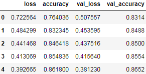
     And that’s it! The neural network is trained. At each epoch during training, Keras displays the number of instances processed so far (along with a progress bar), the mean training time per sample, and the loss and accuracy (or any other extra metrics you asked for) on both the training set and the validation set. You can see that the training loss went down, which is a good sign, and the validation accuracy reached 89.24% after 30 epochs. That’s not too far from the training accuracy, so there does not seem to be much overfitting going on.

############################
Note
     Instead of passing a validation set using the validation_data argument, you could set validation_split to the ratio of the training set that you want Keras to use for validation. For example, validation_split=0.1 tells Keras to use the last 10% of the data (before shuffling) for validation.
############################

• If the training set was very skewed, with some classes being overrepresented(代表过多) and others underrepresented(代表性不足), it would be useful to set the class_weight argument when calling the fit() method, which would give a larger weight to underrepresented classes and a lower weight to overrepresented classes. These weights would be used by Keras when computing the loss.
   
• If you need per-instance weights, set the sample_weight argument
   
• (if both class_weight and sample_weight are provided, Keras multiplies them).
   
• Per-instance weights could be useful if some instances were labeled by experts while others were labeled using a crowdsourcing众包 platform: you might want to give more weight to the former.
   
• You can also provide sample weights (but not class weights) for the validation set by adding them as a third item in the validation_data tuple.

     The fit() method returns

1. a History object containing the training parameters (history.params),

   history.params

   

   import math
   
   math.ceil(55000/history.params["batch_size"])

   

2. the list of epochs it went through (history.epoch),

   print( history.epoch )

   
3. and most importantly a dictionary (history.history) containing the loss and extra metrics it measured at the end of each epoch on the training set and on the validation set (if any).

   history.history.keys()

   
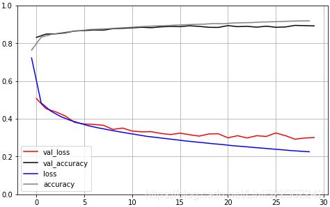
   If you use this dictionary to create a pandas DataFrame and call its plot() method, you get the learning curves shown in Figure 10-12:

   pd.DataFrame(history.history).head()

   

   import pandas as pd
   import matplotlib.pyplot as plt
    
   colors=["blue", "gray", # train_loss      accuracy
           "red", "black"] #   val_loss  val_accuracy
   
   pd.DataFrame( history.history).plot(figsize=(8,5), color=colors)
   plt.grid(True)
   plt.gca().set_ylim(0,1) # set the vertical range to [0-1]
   plt.show()

        Figure 10-12. Learning curves: the mean training loss and accuracy measured over each epoch, and the mean validation loss and accuracy measured at the end of each epoch 

   

     You can see that both the training accuracy and the validation accuracy steadily increase during training, while the training loss and the validation loss decrease. Good! Moreover, the validation curves are close to the training curves, which means that there is not too much overfitting. In this particular case, the model looks like it performed better on the validation set than on the training set at the beginning of training. But that’s not the case: indeed, the validation error is computed at the end of each epoch, while the training error is computed using a running mean during each epoch. So the training curve should be shifted by half an epoch to the left. If you do that, you will see that the training and validation curves overlap almost perfectly at the beginning of training.

Note: DataFrame.shift( periods=int ,axis=0) means only shift integer unit when axis=0

import pandas as pd
import matplotlib.pyplot as plt
 
colors=[#"blue", "gray", #  loss      accuracy
        "red", "black"] #   val_loss  val_accuracy
                               #df[ ["val_loss","val_accuracy"] ].plot(figsize=(8,5), color=colors)
pd.DataFrame( history.history )[["val_loss","val_accuracy"]].plot(figsize=(8,5), color=colors)
#shift(-0.5)
         #1D array                #list
plt.plot(np.arange(-0.5,29,1), history.history["loss"], c="blue", label="loss")    #must be put after previous code for plotting Dataframe
plt.plot(np.arange(-0.5,29,1), history.history["accuracy"], c="gray", label="accuracy")#must be put after previous code for plotting Dataframe
plt.legend()
plt.grid(True)
plt.gca().set_ylim(0,1) # set the vertical range to [0-1]
plt.show()

 

#################
Note
     When plotting the training curve, it should be shifted by half an epoch to the left.
#################

     The training set performance ends up beating the validation performance, as is generally the case when you train for long enough. You can tell that the model has not quite converged yet, as the validation loss is still going down, so you should probably continue training. It’s as simple as calling the fit() method again, since Keras just continues training where it left off (you should be able to reach close to 89% validation accuracy).

     If you are not satisfied with the performance of your model, you should go back and tune the hyperparameters. The first one to check is the learning rate. If that doesn’t help, try another optimizer (and always retune the learning rate after changing any hyperparameter). If the performance is still not great, then try tuning model hyper‐parameters such as the number of layers, the number of neurons per layer, and the types of activation functions to use for each hidden layer. You can also try tuning other hyperparameters, such as the batch size (it can be set in the fit() method using the batch_size argument, which defaults to 32). We will get back to hyperparameter tuning at the end of this chapter. Once you are satisfied with your model’s validation accuracy, you should evaluate it on the test set to estimate the generalization error before you deploy the model to production. You can easily do this using the evaluate() method (it also supports several other arguments, such as batch_size and sample_weight; please check the documentation for more details):

model.evaluate( X_test, y_test )

   

     As we saw in Chapter 2, it is common to get slightly lower performance on the test set than on the validation set, because the hyperparameters are tuned on the validation set, not the test set (however, in this example, we did not do any hyperparameter tuning, so the lower accuracy is just bad luck). Remember to resist the temptation to tweak the hyperparameters on the test set, or else your estimate of the generalization error will be too optimistic.

Using the model to make predictions

     Next, we can use the model’s predict() method to make predictions on new instances. Since we don’t have actual new instances, we will just use the first three instances of the test set:

X_new = X_test[:3]
y_proba = model.predict(X_new)
y_proba.round(2)

array([[0.  , 0.  , 0.  , 0.  , 0.  , 0.  , 0.  , 0.01, 0.  , 0.98],
       [0.  , 0.  , 0.99, 0.  , 0.01, 0.  , 0.  , 0.  , 0.  , 0.  ],
       [0.  , 1.  , 0.  , 0.  , 0.  , 0.  , 0.  , 0.  , 0.  , 0.  ]],
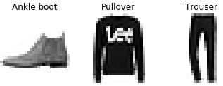
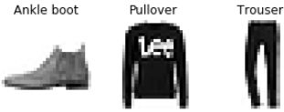
      dtype=float32)

     As you can see, for each instance the model estimates one probability per class, from class 0 to class 9. For example, for the first image it estimates that the probability of class 9 (ankle boot) is 98%, the probability of class 5 (sandal) is 0%, the probability of class 7 (sneaker) is 1%, and the probabilities of the other classes are negligible微不足道的. In other words, it “believes” the first image is footwear, most likely ankle boots but possibly sandals or sneakers. If you only care about the class with the highest estimated probability (even if that probability is quite low), then you can use the predict_classes() method instead:

y_pred = model.predict_classes(X_new)
y_pred

np.array( class_names )[y_pred] 

     Here, the classifier actually classified all three images correctly (these images are shown in Figure 10-13):

y_new = y_test[:3]
y_new

https://blog.csdn.net/Linli522362242/article/details/103786116  : plot_digits 

import matplotlib as mpl
    
def plot_images(instances, target, images_per_row=10, **options):
    size = instances.shape[1] # 28
    images_per_row = min( instances.shape[0], images_per_row )
    n_rows = (instances.shape[0]-1) //images_per_row + 1#or (49-1)//10+1=5 instead 49//10=4 : need +1
                                                        #or (52-1)//10+1=6 instead 52//10=5 # need +1
                                                        #or (50-1)//10+1=5 instead (50)//10+1=6 need 50-1       
    n_cols=images_per_row
    index=0
    for row in range(n_rows):
        for col in range(n_cols):
           plt.subplot(n_rows, images_per_row, index+1)
           plt.imshow(instances[index], cmap="binary", interpolation="nearest")
           plt.axis('off')
           plt.title(class_names[target[index]])
           index += 1 
        rest = instances.shape[0]-index
        if rest==0:
            break
        else:
            n_cols = min( rest, images_per_row )
            
# slice=100
plt.figure( figsize=( min(18, 18*( X_new.shape[0]/10.0 )),  max( 3, 2.9*( X_new.shape[0]/10.0 ))
                    )
          )
# plot_images(X_test[:slice], y_test[:slice],images_per_row=10)
# plt.subplots_adjust(wspace=0.2, hspace=0.5)

plot_images(X_new, y_new )
plt.show()

slice=31
plt.figure( figsize=( min(18, 18*( X_test[:slice].shape[0]/10.0 )),  max( 3, 2.9*( X_test[:slice].shape[0]/10.0 ))
                    )
          )
plot_images(X_test[:slice], y_test[:slice] )
plt.show()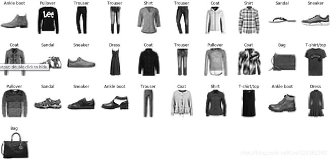

####################################

import tensorflow as tf
from tensorflow import keras

tf.__version__

 

keras.__version__

 

fashion_mnist = keras.datasets.fashion_mnist
(X_train_full, y_train_full), (X_test, y_test) = fashion_mnist.load_data()

X_train_full.shape

      #every image is represented as a 28 × 28 array rather than a 1D array of size 784.

X_train_full.dtype

 
     Note that the dataset is already split into a training set and a test set, but there is no validation set, so we’ll create one now. Additionally, since we are going to train the neural network using Gradient Descent, we must scale the input features. For simplicity, we’ll scale the pixel intensities down to the 0–1 range by dividing them by 255.0 (this also converts them to floats):

# scale the pixel intensities down to the 0–1 range by dividing them by 255.0 (this also converts them to floats)
X_valid, X_train = X_train_full[:5000]/255. , X_train_full[5000:]/255.
y_valid, y_train = y_train_full[:5000], y_train_full[5000:]
X_test = X_test/255.

import pandas as pd
pd.DataFrame(X_train[0])

 

import matplotlib.pyplot as plt
plt.imshow(X_train[0], cmap="binary")
plt.axis("off")
plt.show()

 

class_names = ["T-shirt/top", "Trouser", "Pullover", "Dress", "Coat","Sandal", "Shirt", 
               "Sneaker", "Bag", "Ankle boot"]

X_train.shape, X_valid.shape, X_test.shape

 
Construction Phase

# using tensorflow version 1.

import tensorflow.compat.v1 as tf

n_inputs = 28*28 #MNIS
n_hidden1 = 300
n_hidden2 = 100
n_outputs = 10

tf.reset_default_graph()

X = tf.placeholder(tf.float32, shape=(None, n_inputs), name="X")

---------------------------------------------------------------------------
RuntimeError                              Traceback (most recent call last)
 in 
----> 1 X = tf.placeholder(tf.float32, shape=(None, n_inputs), name="X")

C:\Anaconda3\envs\tensorflow\lib\site-packages\tensorflow_core\python\ops\array_ops.py in placeholder(dtype, shape, name)
   2713   """
   2714   if context.executing_eagerly():
-> 2715     raise RuntimeError("tf.placeholder() is not compatible with "
   2716                        "eager execution.")
   2717 

RuntimeError: tf.placeholder() is not compatible with eager execution.

Solution:

tf.compat.v1.disable_eager_execution()

      Next, just like you did in https://blog.csdn.net/Linli522362242/article/details/106214525, you can use placeholder nodes to represent the training data and targets. The shape of X is only partially defined. We know that it will be a 2D tensor (i.e., a matrix), with instances along the first dimension and features along the second dimension, and we know that the number of features is going to be 28 x 28 (one feature per pixel), but we don't know yet how many instances each training batch will contain. So the shape of X is (None, n_inputs). Similarly, we know that y will be a 1D tensor with one entry per instance, but again we don't know the size of the training batch at this point, so the shape of y is (None).

X = tf.placeholder(tf.float32, shape=(None, n_inputs), name="X")
y = tf.placeholder(tf.int32, shape=(None), name="y")

      Now let's create the actual neural network. The placeholder X will act as the input layer; during the execution phase, it will be replaced with one training batch at a time (note that all the instances in a training batch will be processed simultaneously by the neural network).

     Now you need to create the two hidden layers and the output layer. The two hidden layers are almost identical: they differ only by the inputs they are connected to and by the number of neurons they contain. The output layer is also very similar, but it uses a softmax activation function instead of a ReLU activation function. So let’s create a neuron_layer() function that we will use to create one layer at a time. It will need parameters to specify the inputs, the number of neurons, the activation function, and the name of the layer:

Let's go through the following code line by line:

1. First we create a name scope using the name of the layer: it will contain all the computation nodes for this neuron layer. This is optional, but the graph will look much nicer in TensorBoard if its nodes are well organized.
    
2. Next, we get the number of inputs by looking up the input matrix’s shape and getting the size of the second dimension (the first dimension is for instances).
    
3. The next three lines create a W variable that will hold the weights matrix. It will be a 2D tensor containing all the connection weights between each input and each neuron; hence, its shape will be (n_inputs, n_neurons). It will be initialized randomly, using a truncated normal (Gaussian) distribution with a standard deviation of (Using a truncated normal distribution rather than a regular normal distribution ensures that there won't be any large weights, which could slow down training. ### truncated_normal( shape, mean=0.0, stdev=1.0 ) # range: [ mean-2*stddev, mean+2*stddev ]###). Using this specific standard deviation helps the algorithm converge much faster (we will discuss this further in Chapter 11; it is one of those small tweaks to neural networks that have had a tremendous impact on their efficiency). It is important to initialize connection weights randomly for all hidden layers to avoid any symmetries that the Gradient Descent algorithm would be unable to break.
    
4. The next line creates a b variable for biases, initialized to 0 (no symmetry issue in this case), with one bias parameter per neuron
    
5. Then we create a subgraph to compute z = X · W + b. This vectorized implementation will efficiently compute the weighted sums of the inputs plus the bias term for each and every neuron in the layer, for all the instances in the batch in just one shot.
    
6. Finally, if the activation parameter is set to "relu", the code returns relu(z) (i.e., max (0, z)), or else it just returns z.

   import numpy as np
   
   #inputs, the number of neurons, the name of the layer, the activation function
   def neuron_layer( X, n_neurons, name, activation=None):
       with tf.name_scope(name):
           n_inputs = int( X.get_shape()[1] ) # X.get_shape()[1] : the number of features
           
           stddev = 2 / np.sqrt( n_inputs )
                                          # shape
           init = tf.truncated_normal( (n_inputs, n_neurons), stddev=stddev )
           # truncated_normal( shape, mean=0.0, stdev=1.0 ) # range: [ mean-2*stddev, mean+2*stddev ]
           # stddev=stddev ==> stddev= 2/np.sqrt( n_inputs ) ==> range: mean += 2* 2/np.sqrt( n_inputs )
           # 截断的产生正态分布的随机数，即随机数与均值的差值若大于两倍的标准差，则重新生成 |x-mean| <=2*stddev
           W = tf.Variable(init, name="kernel")                # W.shape: (features, n_neurons)
           b = tf.Variable(tf.zeros([n_neurons]), name="bias")
           Z = tf.matmul( X,W) # X dot W # prediction          # X.shape(): (instances, features)  
                                                               # X dot W ==> Z.shape(instances, n_neurons) 
           if activation is not None:
               return activation(Z)
           else:
               return Z

   #n_inputs = 28*28+1 ==> n_hidden1 = 300 ==> n_hidden2 = 100 ==> n_outputs = 10
   with tf.name_scope("dnn"):
       hidden1 = neuron_layer( X, n_hidden1, name="hidden1", activation=tf.nn.relu )
       hidden2 = neuron_layer( hidden1, n_hidden2, name="hidden2", activation=tf.nn.relu )
       logits = neuron_layer( hidden2, n_outputs, name="outputs" )

    Notice that once again we used a name scope for clarity清晰度. Also note that logits is the output of the neural network before going through the softmax activation function: for optimization reasons, we will handle the softmax computation later. ==>==>

   with tf.name_scope("loss"):
       xentropy = tf.nn.sparse_softmax_cross_entropy_with_logits( labels=y, logits=logits )
       loss = tf.reduce_mean( xentropy, name="loss")

    The sparse_softmax_cross_entropy_with_logits() function is equivalent to applying the softmax activation function###  return index/k max of  ###and then computing the cross entropy(minimize + to get ), but it is more efficient, and it properly takes care of corner cases like logits equal to 0 (-infinity).

   learning_rate = 0.01
   with tf.name_scope("train"):
       optimizer = tf.train.GradientDescentOptimizer( learning_rate )
       training_op = optimizer.minimize(loss)

   Cross entropy cost function + 

   an additional  penalty: 

   Then Cross entropy gradient vector for class k ,  (this equation also has to add a step for containing the case of i=0 for bias)

     is a weight vector: Theta = Theta - eta*gradients   , eta is the learning rate 

   with tf.name_scope("eval"):
       #k=1 is the top-one class  # tf.nn.in_top_k(predictions, targets, k, name=None)
       correct = tf.nn.in_top_k( logits, y, 1) #logits.shape : (samples, class_dimensions)
       accuracy = tf.reduce_mean( tf.cast(correct, tf.float32) )

   And, as usual, we need to create a node to initialize all variables, and we will also create a Saver to save our trained model parameters to disk:

   init = tf.global_variables_initializer()
   saver = tf.train.Saver()

    

Execution Phase

# since we want to use two dimentions of dataset (instances, 784)

X_train = X_train.astype(np.float32).reshape(-1, 28*28)
X_valid = X_valid.astype(np.float32).reshape(-1, 28*28)
X_test = X_test.astype(np.float32).reshape(-1, 28*28)

Now we define the number of epochs that we want to run, as well as the size of the mini-batches: 

n_epochs = 40
batch_size = 50

     I want to make sure that the instances are picked randomly, but some instances may be picked serveral times per epoch/loop while others may not be picked at all, so I shuffle the dataset, then go through it instance by instance.

def shuffle_batch( X, y, batch_size ):
    rnd_idx = np.random.permutation( len(X) )
    n_batches = len(X) // batch_size
    # np.array_split(rnd_idx, n_batches) # split the list of rnd_idx to n_batches groups
    for batch_idx in np.array_split(rnd_idx, n_batches):
        X_batch, y_batch = X[batch_idx], y[batch_idx]
        yield X_batch, y_batch

with tf.Session() as sess:
    init.run()
    for epoch in range(n_epochs):
        for X_batch, y_batch in shuffle_batch( X_train, y_train, batch_size ):
            sess.run(training_op, feed_dict={X: X_batch, y:y_batch})
        # Next, at the end of each epoch, the code evaluates the model on the last mini-batch 
        # and on the full validation set, and it prints out the result.    
        acc_batch = accuracy.eval(feed_dict={X: X_batch, y:y_batch})
        acc_val = accuracy.eval( feed_dict={X: X_valid, y: y_valid} )
        print( epoch, "(Last) Batch accuracy: ", acc_batch, "~ Val accuracy: ", acc_val )
    save_path = saver.save(sess, "./my_model_final.ckpt") # Finally, the model parameters are saved to disk.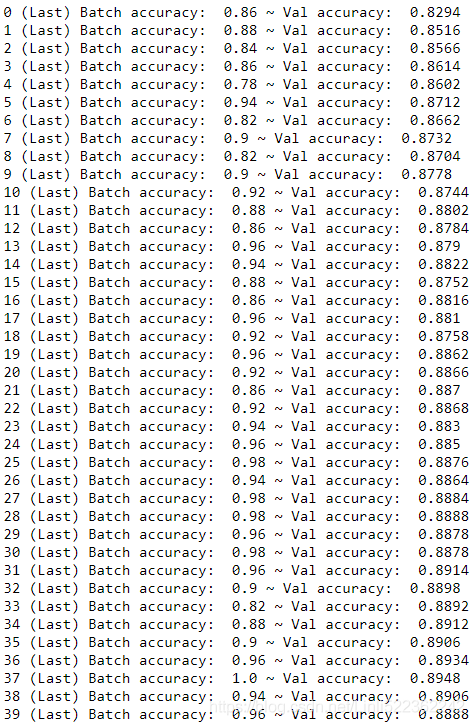

  It seems overfit, but I just want to show how does the neunon work.

import os
os.environ["PATH"] += os.pathsep + "C:/Graphviz2.38/bin" # " directory" where you intall graphviz
 
import tfgraphviz as tfg
 
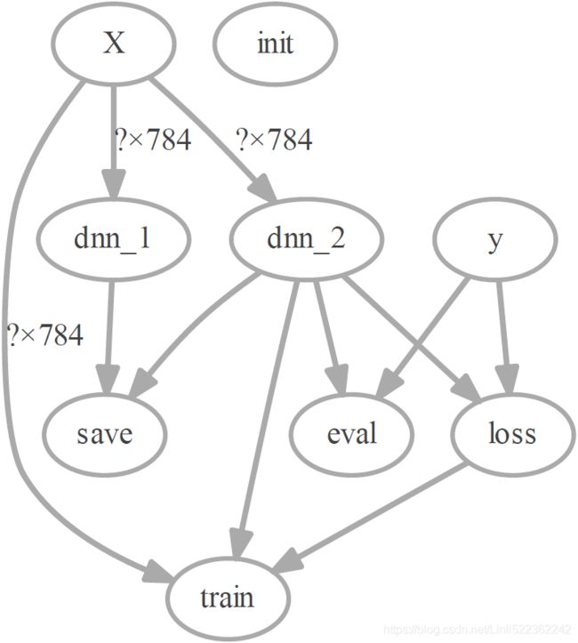
tfg.board( tf.get_default_graph() ).view()

 

 Using the Neural Network

     Now that the neural network is trained, you can use it to make predictions. To do that, you can reuse the same construction phase, but change the execution phase like this:

with tf.Session() as sess:
    saver.restore( sess, "./my_model_final.ckpt" ) # or better, use save_path
    X_new = X_test[:3]  #######
    Z = logits.eval( feed_dict={X: X_new } )
    y_pred = np.argmax( Z, axis=1 )

y_pred

np.array( class_names )[y_pred] 

 
Equation 4-20. Softmax function 

np.exp( np.max(Z, axis=1) ) / np.sum(np.exp(Z), axis=1)

 

y_new = y_test[:3]
y_new

 

import matplotlib as mpl
    
def plot_images(instances, target, images_per_row=10, **options):
    size = instances.shape[1] # 28
    images_per_row = min( instances.shape[0], images_per_row )
    n_rows = (instances.shape[0]-1) //images_per_row + 1#or (49-1)//10+1=5 instead 49//10=4 : need +1
                                                        #or (52-1)//10+1=6 instead 52//10=5 # need +1
                                                        #or (50-1)//10+1=5 instead (50)//10+1=6 need 50-1       
    n_cols=images_per_row
    index=0
    for row in range(n_rows):
        for col in range(n_cols):
           plt.subplot(n_rows, images_per_row, index+1)
           plt.imshow(instances[index].reshape(28,28), cmap="binary", interpolation="nearest")
           plt.axis('off')
           plt.title(class_names[target[index]])
           index += 1 
        rest = instances.shape[0]-index
        if rest==0:
            break
        else:
            n_cols = min( rest, images_per_row )
            
# slice=100
plt.figure( figsize=( min(18, 18*( X_new.shape[0]/10.0 )),  max( 3, 2.9*( X_new.shape[0]/10.0 ))
                    )
          )
# plot_images(X_test[:slice], y_test[:slice],images_per_row=10)
# plt.subplots_adjust(wspace=0.2, hspace=0.5)

plot_images(X_new, y_new )
plt.show()

 

####################################

      Now you know how to use the Sequential API to build, train, evaluate, and use a classification MLP. But what about regression?

Building a Regression MLP Using the Sequential API

https://blog.csdn.net/Linli522362242/article/details/106582512