【数据分析】时变参数随机波动率向量自回归模型（TVP-VAR）

一、

VAR:向量自回归模型，结果仅具有统计上的 意义

SVAR：结构向量自回归模型

TVP-VAR：Time Varying Parameter-Stochastic Volatility-Vector Auto Regression。时变参数随机波动率向量自回归模型，与VAR 不同的是，模型没有同方差的假定，更符合实际。并且时变参数假定随机波动率，更能捕捉到经济变量在不同时代背景下所具有的关系和特征（时变影响）。将随机波动性纳入TVP估算中可以显着提高估算性能。在VAR模型中，所有的参数遵循一阶游走过程。

      随机波动的概念在TVP-VAR中很重要，随机波动是1976年由Black提出，随后在经济计量中有很大的发展。近几年，随机波动也经常被用在宏观经济的经验分析中。很多情况下，经济数据的产生过程中具有漂移系数和随机波动的冲击，如果是这种情况，那么使用具有时变系数但具有恒定波动性的模型会引起一个问题，即由于忽略了扰动中波动性的可能变化，估计的时变系数可能会出现偏差。为了避免这种问题，TVP-VAR模型假设了随机波动性。尽管似然函数难以处理，所以随机波动率使估计变得困难，但是可以在贝叶斯推断中使用马尔可夫链蒙特卡罗（MCMC）方法来估计模型。

从 具有随机波动性的时变参数（TVP）回归模型的估计算法(TVP-VAR模型的单变量情况)说起。

 

 是反应的标量，是k×1的协变量向量，是p×1的协变量向量。β是k×1的常系数向量；是p×1的时变向量；是随机波动。

假设=0，。

 式1中，β部分是常系数向量，对的影响是假设不随时间变化而变化的；部分是时变向量，假设对的回归关系是时变的。

 时变系数假设遵循式2中的一阶随机游走过程。漂移系数可以捕获可能存在的非线性，例如结构破坏。也就是说，时变系数可以捕获真正的移动以及虚假移动。也就是说，如果和的关系不清楚，可能会出现过拟合。

对于回归的干扰项，服从随时间变化的正态分布。对数波动率。

 

　

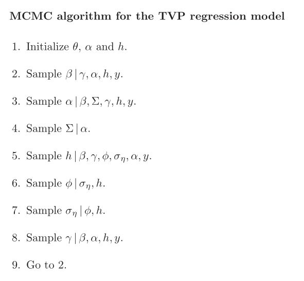
二、MCMC算法

MCMC算法，一种随机采样方法，即蒙特卡罗方法（Monte Carlo Simulation，简称MC）和马尔科夫链（Markov Chain ，也简称MC）。MCMC方法是用来在概率空间，通过随机采样估算兴趣参数的后验分布。

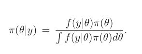
MCMC方法是在贝叶斯推断的背景下考虑的，其目标是在研究人员预先设定的特定先验概率密度下评估目标参数的联合后验分布。

在贝叶斯推断中，为未知参数θ的向量指定先验密度，用π（θ）表示。用f(y|θ)表示数据y = {y 1 ,...,y n }的似然函数。然后根据先验分布进行推断，用 π(θ|y)表示。

MCMC算法通过递归采样条件后验分布来进行，其中在仿真中使用了条件参数的最新值。

Gibbs采样器是著名的MCMC方法之一。步骤如下：

 

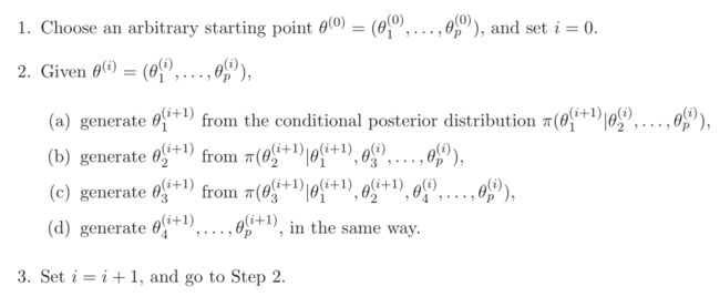
对于MCMC算法，π(θ)为先验密度，后验分布 π(θ,α,h|y）^4。

(具体参数参考Nakajima原文)

 

三、TVP-VAR Model

首先考虑SVAR model的定义：

yt是k×1的观察变量，A，F是k×k的系数矩阵，扰动项ut是k×1的结构性冲击，假设，

 

 

 

 假设A为下三角矩阵，通过递归识别指定结构冲击的关系。

 

 

所以，式6可以写为：

其中，，定义，（ Kronecker乘积）。

 

 

                                      （7）

 

 

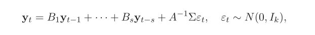
 式7中，所有的参数都是时变的。所以，TVP-VAR模型：

                                （8）

，，都是时变的。

是下三角矩阵，

 

式8中的参数都遵循以下随机游走过程：

 

 

 注意：

1.假设参数服从随机游走过程

2.时变参数的方差和协方差结构由参数控制。许多文章中假定是对角矩阵。

 

3.当在贝叶斯推断中实现TVP-VAR模型时，应谨慎选择先验，因为TVP-VAR模型具有许多状态变量，并且其过程被建模为非平稳随机游走过程TVP-VAR模型非常灵活，状态变量可以捕捉潜在经济结构的渐进和突变。但是在VAR模型中的每个参数中允许时间变化可能会导致过度识别问题。

 

 

四、进行TVP-VAR建模时，也需要数据平稳。可以用ADF单位根检验法检验数据的平稳性，不平稳的数据可以做差分，直至平稳，用差分后的数据进行建模。

需要注意的是：TVP-VAR建模时，变量之间的顺序会影响到最后的实证结果。变量的顺序问题可能是实证结果不符合预期的一个原因。最好把关注的变量放在首位，这样在时变关系图中就能得到较好的展示。

%==================================4.1 Main================================
clear;
clc;

% Load Korobilis (2008) quarterly data
load ydata.dat; % data 
load yearlab.dat; % data labels 

%%
%----------------------------------BASICS----------------------------------


Y=ydata;
t=size(Y,1);        % t - The total number of periods in the raw data (t=215)
M=size(Y,2);        % M - The dimensionality of Y (i.e. the number of variables)(M=3)
tau = 40;           % tau - the size of the training sample (the first forty quarters)
p = 2;              % p - number of lags in the VAR model 

%% Generate the Z_t matrix, i.e. the regressors in the model. 

ylag = mlag2(Y,p);          % This function generates a 215x6 matrix with p lags of variable Y. 
ylag = ylag(p+tau+1:t,:);   % Then remove our training sample, so now a 173x6 matrix. 

K = M + p*(M^2);            % K is the number of elements in the state vector

% Here we distribute the lagged y data into the Z matrix so it is
% conformable with a beta_t matrix of coefficients. 

Z = zeros((t-tau-p)*M,K);   
for i = 1:t-tau-p
    ztemp = eye(M);
    for j = 1:p        
        xtemp = ylag(i,(j-1)*M+1:j*M); 
        xtemp = kron(eye(M),xtemp);
        ztemp = [ztemp xtemp];
    end
    Z((i-1)*M+1:i*M,:) = ztemp;
end

% Redefine our variables to exclude the training sample and the first two
% lags that we take as given, taking total number of periods (t) from 215 
% to 173. 

y = Y(tau+p+1:t,:)';
yearlab = yearlab(tau+p+1:t);
t=size(y,2); % t now equals 173

%% --------------------MODEL AND GIBBS PRELIMINARIES-----------------------

nrep = 5000;    % Number of sample draws 
nburn = 2000;   % Number of burn-in-draws
it_print = 100; % Print in the screen every "it_print"-th iteration


%% INITIAL STATE VECTOR PRIOR  

% We use the first 40 observations (tau) to run a standard OLS of the
% measurement equation, using the function ts_prior. The result is
% estimates for priors for B_0 and Var(B_0). 

[B_OLS,VB_OLS]= ts_prior(Y,tau,M,p);

% Given the distributions we have, we now have to define our priors for B,
% Q and Sigma. These are set in accordance with how they are set in 
% Primiceri (2005). These are the hyperparameters of the beta, Q and Sigma
% initial priors. 

B_0_prmean = B_OLS;
B_0_prvar = 4*VB_OLS; 

Q_prmean = ((0.01).^2)*tau*VB_OLS;
Q_prvar = tau;

Sigma_prmean = eye(M);
Sigma_prvar = M+1;

% To start the Kalman filtering assign arbitrary values that are in support
% of their priors, Q and Sigma. 

consQ = 0.0001;
Qdraw = consQ*eye(K);
Sigmadraw = 0.1*eye(M);

% Create some matrices for storage that will be filled in once we
% start the Gibbs sampling.

Btdraw = zeros(K,t); 
Bt_postmean = zeros(K,t);
Qmean = zeros(K,K);
Sigmamean = zeros(M,M);

%% -------------------------IRF-PRELIMINARIES------------------------------
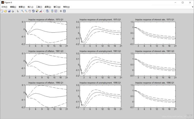
nhor = 21;     % The number of periods in the impulse response function. 

% Matricies to be filled containing IRFs for 1975q1, 1981q3, 1996q1. The 
% dimensions correspond to the iterations of the gibbs sample, each of the
% variables, and each of the 21 periods of the IRF analysis. 

imp75 = zeros(nrep,M,nhor); 
imp81 = zeros(nrep,M,nhor);
imp96 = zeros(nrep,M,nhor);

% This corresponds to variable J introduced in equation (14) in the report

bigj = zeros(M,M*p); 
bigj(1:M,1:M) = eye(M);


%% ================ START GIBBS SAMPLING ==================================

tic; % This is just a timer
disp('Number of iterations');


for irep = 1:nrep + nburn    % 7000 gibbs iterations starts here
    % Print iterations - this just updates on the progress of the sampling
    if mod(irep,it_print) == 0
        disp(irep);toc;
    end
    
%% Draw 1: B_t from p(B_t|y,Sigma)
    
    % We use the function 'carter_kohn_hom' to to run the FFBS algorithm. 
    % This results in a 21x173 matrix, corresponding to one Gibbs sample
    % draw of each of the coefficients in each time period. The inputs
    % Sigmadraw and Qdraw are updated for each Gibbs sample repetition.
    
    [Btdraw] = carter_kohn_hom(y,Z,Sigmadraw,Qdraw,K,M,t,B_0_prmean,B_0_prvar);
    
  
%% Draw 2: Q from p(Q^{-1}|y,B_t) which is i-Wishart

    % We draw Q from an Inverse Wishart distribution. The parameters 
    % of the distribution are derived as equation (11) in the main report.
    % The mean is taken as the inverse of the accumulated sum of squared 
    % errors added to the prior mean, and the variance is simply t.  
    
    % Differencing Btdraw to create the sum of squared errors
    
    Btemp = Btdraw(:,2:t)' - Btdraw(:,1:t-1)'; 
    sse_2Q = zeros(K,K);
    for i = 1:t-1
        sse_2Q = sse_2Q + Btemp(i,:)'*Btemp(i,:);
    end

    Qinv = inv(sse_2Q + Q_prmean);      % compute mean to use for Wishart draw
    Qinvdraw = wish(Qinv,t+Q_prvar);    % draw inv q from the wishart distribution
    Qdraw = inv(Qinvdraw);              % find non-inverse q 
    
%% Draw 3: Sigma from p(Sigma|y,B_t) which is i-Wishart

    % We draw Sigma from an Inverse Wishart distribution. The parameters 
    % of the distirbution are derived as equation (10) in the main report. 
    % The mean is taken as the inverse of the sum of squared residuals
    % added to the prior mean. The variance is simply t. 
    
    % Find residuals using data and the current draw of coefficients
    
    resids = zeros(M,t);
    for i = 1:t
        resids(:,i) = y(:,i) - Z((i-1)*M+1:i*M,:)*Btdraw(:,i);
    end
    
    % Create a matrix for the accumulated sum of squared residuals, to
    % be used as the mean parameter in the i-Wishart draw below. 
    sse_2S = zeros(M,M);
    for i = 1:t
        sse_2S = sse_2S + resids(:,i)*resids(:,i)';
    end
    
    Sigmainv = inv(sse_2S + Sigma_prmean);          % compute mean to use for the Wishart
    Sigmainvdraw = wish(Sigmainv,t+Sigma_prvar);    % draw from the Wishsart distribution
    Sigmadraw = inv(Sigmainvdraw);                  % turn into non-inverse Sigma
    
%% IRF 
    % We only apply IRF analysis once we have exceeded the burn-in draws phase.
    if irep > nburn;         
            
            % Create matrix that is going to contain all beta draws over
            % which we will take the mean after the Gibbs sampler as our moment
            % estimate: 
            Bt_postmean = Bt_postmean + Btdraw;
            
            % biga is the A matrix of the VAR(1) version of our VAR(2) model, 
            % found in equation (12. biga changes in every period of the 
            % analysis, because the coefficients are time varying, so we 
            % apply the analysis below in every time period. 
            
            biga = zeros(M*p,M*p); 
            for j = 1:p-1
                biga(j*M+1:M*(j+1),M*(j-1)+1:j*M) = eye(M); % fill the A matrix with identity matrix (3) in bottom left corner
            end

            % The following procedure is applied separately in each time period. 
            
            % This loop takes coefficients of the relevant time period from
            % Bt_draw (which contains all coefficients for all t) and uses
            % them to update the biga matrix, so that it can change for
            % every t. 
            
            for i = 1:t 
                bbtemp = Btdraw(M+1:K,i);  % get the draw of B(t) at time i=1,...,T  (exclude intercept)
                splace = 0;
                for ii = 1:p
                    for iii = 1:M
                        biga(iii,(ii-1)*M+1:ii*M) = bbtemp(splace+1:splace+M,1)'; % Load non-intercept coefficient draws
                        splace = splace + M;
                    end
                end
                
                % Next we want to create a shock matrix in which the third
                % column is [0 0 1]', therefore implementing a unit shock
                % in the interest rate. 
                
                shock = eye(3);
                
                % Now get impulse responses for 1 through nhor future
                % periods. impresp is a 3x63 matrix which contains 9
                % response values in total for each period, 3 for each 
                % variable. These three responses correspond to the 3
                % possible shocks that are contained in the schock
                % matrix
                
                % bigai is updated through mulitiplication with the 
                % coefficient matrix after each time period. 
                                
                % Create a results matrix to store impulse responses in all periods
                impresp = zeros(M,M*nhor); 
                
                % Fill in the first period of the results matrix with the shock (as defined above) 
                impresp(1:M,1:M) = shock;
                
                % Create a separate variable for the a matrix so that we
                % can update it for each period of the IRF analysis. 
                bigai = biga; 
                
                % This follows the impulse response function as in equation 15.
                % Fill in each period of the results matrix according to
                % the impulse response function formula. 
                
                for j = 1:nhor-1
                    impresp(:,j*M+1:(j+1)*M) = bigj*bigai*bigj'*shock;
                    bigai = bigai*biga; % update the coefficient matrix for next period
                end

                % The section below keeps only the responses that we are interested in:
                % - those from the periods 1975q1, 1981q3, and 1996q1
                % - those that correspond to the shock in the interest 
                % rate (i.e. those caused by the third column of our shock
                % matrix). 
                
                if yearlab(i,1) == 1975.00;   % store only IRF from 1975:Q1
                    impf_m = zeros(M,nhor);
                    jj=0;
                    for ij = 1:nhor
                        jj = jj + M;    % select only the third column for each time period of the IRF
                        impf_m(:,ij) = impresp(:,jj);
                    end           
                % For each iteration of the Gibbs sampler, fill in the
                % results along the first dimension 
                    imp75(irep-nburn,:,:) = impf_m; 
                end
                
                if yearlab(i,1) == 1981.50;   % store only IRF from 1981:Q3
                    impf_m = zeros(M,nhor);
                    jj=0;
                    for ij = 1:nhor
                        jj = jj + M;    % select only the third column for each time period of the IRF
                        impf_m(:,ij) = impresp(:,jj);
                    end
                % For each iteration of the Gibbs sample, fill in the
                % results along the first dimension 
                    imp81(irep-nburn,:,:) = impf_m; 
                end
                
                if yearlab(i,1) == 1996.00;   % store only IRF from 1996:Q1
                    impf_m = zeros(M,nhor);
                    jj=0;
                    for ij = 1:nhor
                        jj = jj + M;    % select only the third column for each time period of the IRF
                        impf_m(:,ij) = impresp(:,jj);
                    end
                % For each iteration of the Gibbs sample, fill in the
                % results along the first dimension 
                    imp96(irep-nburn,:,:) = impf_m; 
                end
            end % End getting impulses for each time period 
        end % End the impulse response calculation section   
end % End main Gibbs loop (for irep = 1:nrep+nburn)

clc;
toc; % Stop timer and print total time
%% ================ END GIBBS SAMPLING ==================================

% Even though it is not used in our IRF analysis since we are integrating
% that into the Gibbs sampling loop, here is how to take the mean of the 
% draw of the betas as moment estimate:

Bt_postmean = Bt_postmean./nrep;

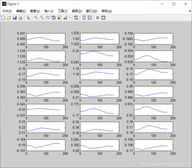
%% Graphs and tables

% This works out the percentage range of that each variable's coefficient
% spans across time. I.e. to what extent was the TVP facility used by each
% variable in the model? This is calculated by finding the range for each
% variable as a percentage of the mean coefficient size for that variable.
% The result is a 21x1 vector, and it is reshaped into a 3x7 matrix in order
% to map onto the system of equations (2,3,and 4) set out in the report.

Bt_range = ones(21,1)
for i = 1:21
    Bt_range(i) = abs((max(Bt_postmean(i,:))-min(Bt_postmean(i,:)))/mean(Bt_postmean(i,:)))
end 
Bt_range = reshape(Bt_range,3,7)
 
% Create a table of coefficient ranges for export to the report

rowNames = {'Inflation','Unemployment','Interest Rate'};
colNames = {'Intercept','Inf_1','Unemp_1', 'IR_1','Inf_2','Unemp_2', 'IR_2'};
pc_change_table = array2table(Bt_range,'RowNames',rowNames,'VariableNames',colNames)
 
writetable(pc_change_table,'pc_change.csv')

% Now plot a separate chart for each of the coefficients
 
figure
for i = 1:21       
    subplot(7,3,i)
    plot(1:t,Bt_postmean(i,:))  
end 

% Now we move to plotting the IRF. This section takes moments along the
% first dimension, i.e. across the Gibbs sample iterations. The moments
% are for the 16th, 50th and 84th percentile. 

    qus = [.16, .5, .84];
    imp75XY=squeeze(quantile(imp75,qus)); 
    imp81XY=squeeze(quantile(imp81,qus));
    imp96XY=squeeze(quantile(imp96,qus));
    
    % Plot impulse responses
    figure       
    set(0,'DefaultAxesColorOrder',[0 0 0],...
        'DefaultAxesLineStyleOrder','--|-|--')
    subplot(3,3,1)
    plot(1:nhor,squeeze(imp75XY(:,1,:)))
    title('Impulse response of inflation, 1975:Q1')
    xlim([1 nhor])
    ylim([-0.2 0.1])
%    % yline(0)
    set(gca,'XTick',0:3:nhor)
    subplot(3,3,2)
    plot(1:nhor,squeeze(imp75XY(:,2,:)))
    title('Impulse response of unemployment, 1975:Q1')
    xlim([1 nhor])
    ylim([-0.2 0.2])
   % yline(0)
    set(gca,'XTick',0:3:nhor)    
    subplot(3,3,3)
    %ylim([0 1])
%    % yline(0)
    plot(1:nhor,squeeze(imp75XY(:,3,:)))
    title('Impulse response of interest rate, 1975:Q1')
    xlim([1 nhor])
    %ylim([-0.3 0.1])
   % yline(0)
    set(gca,'XTick',0:3:nhor)    
    subplot(3,3,4)
    plot(1:nhor,squeeze(imp81XY(:,1,:)))
    title('Impulse response of inflation, 1981:Q3')
    xlim([1 nhor])
    ylim([-0.2 0.1])
   % yline(0)
    set(gca,'XTick',0:3:nhor)    
    subplot(3,3,5)
    plot(1:nhor,squeeze(imp81XY(:,2,:)))
    title('Impulse response of unemployment, 1981:Q3')
    xlim([1 nhor])
    ylim([-0.2 0.2])
   % yline(0)
    set(gca,'XTick',0:3:nhor)    
    subplot(3,3,6)
    plot(1:nhor,squeeze(imp81XY(:,3,:)))
    title('Impulse response of interest rate, 1981:Q3')
    xlim([1 nhor])
    %ylim([-0.4 0.1])
   % yline(0)
    set(gca,'XTick',0:3:nhor)    
    subplot(3,3,7)
    plot(1:nhor,squeeze(imp96XY(:,1,:)))
    title('Impulse response of inflation, 1996:Q1')
    xlim([1 nhor])
    ylim([-0.2 0.1])
   % yline(0)
    set(gca,'XTick',0:3:nhor)    
    subplot(3,3,8)
    plot(1:nhor,squeeze(imp96XY(:,2,:)))
    title('Impulse response of unemployment, 1996:Q1')
    xlim([1 nhor])
    ylim([-0.2 0.2])
   % yline(0)
    set(gca,'XTick',0:3:nhor)
    subplot(3,3,9)
    plot(1:nhor,squeeze(imp96XY(:,3,:)))
    title('Impulse response of interest rate, 1996:Q1')
    xlim([1 nhor])
     %ylim([0 1])
    % yline(0)
    set(gca,'XTick',0:3:nhor)
    
disp('             ')
disp('To plot impulse responses, use:         plot(1:nhor,squeeze(imp75XY(:,VAR,:)))           ')
disp('             ')
disp('where VAR=1 for impulses of inflation, VAR=2 for unemployment and VAR=3 for interest rate')

完整代码添加QQ1575304183