深度学习03: CNN经典网络LeNet, AlexNet, VGG-16解读
计算机视觉研究中的大量研究,都集中在如何把卷积层,池化层,全连接层这些基本构件组合起来,形成有效的卷积神经网络;
找设计灵感的最好方法之一,就是去看一些案例,就像学习编程一样,通过研究别人构建有效组件的案例,是个不错的方法;
实际上,在计算机视觉任务中表现良好的神经网络框架,往往也适用于其它任务。
一些经典的神经网络架构范例,当中的一些思路为现代计算机视觉技术的发展奠定了基础。
经典网络: LeNet-5、AlexNet、VGG、ResNet(152层)
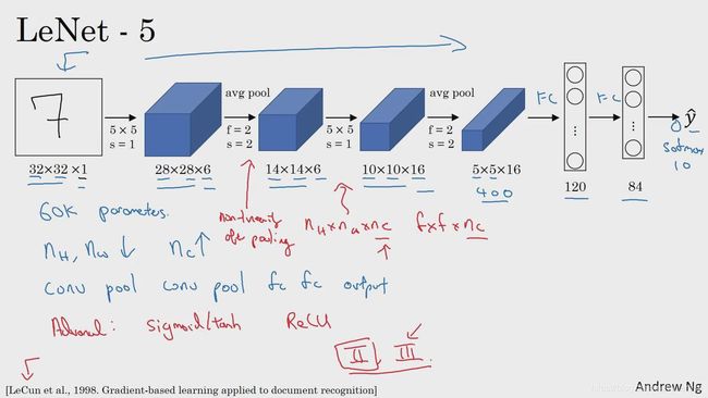
1.LeNet-5
paper:http://yann.lecun.com/exdb/publis/pdf/lecun-98.pdf
注:大约6万参数
1.该网络诞生的年代(1980年代),流行用平均池化,现在更常用的是最大池化;
2.当时并不使用padding;
3.现代版本,最后输出用softmax;
总的来说:
从左到右,随着网络越来越深,图像的宽高在减少,而信道数量在增加;
网络模式,一个或多个卷积层后面跟着一个池化层,然后又是若干个卷积层,再接一个池化层,然后是全连接层,最后是输出,这种排列方式很常用。
阅读经典论文:
读这篇经典论文时,你会发现过去认识使用sigmoid函数和tanh函数,而不是ReLu函数;这种网络特别之处在于,各网络层之间是有关联的;
建议精度第二,泛读第三段
2. AlexNet
https://papers.nips.cc/paper/4824-imagenet-classification-with-deep-convolutional-neural-networks.pdf
注:大约6000万参数
1.原文是224x224,但实际227x227效果更好一些;
2.AlexNet实际上跟LeNet有很多相似之处,不过AlexNet要大得多;它性能优于LeNet主要原因有:
a.含有大量隐藏单元;
b.使用了ReLu激活单元;
3.写这篇论文时,GPU还很慢,所以AlexNet采用了非常复杂的方法在2个GPU上训练,
大致原理是这些层被分拆到2个GPU中运行,还专门设计一个方法用于两个GPU的通信;
经典的AlexNet网络,还有另一种类型的层,“局部响应归一化层”,即LRN层;这类层应用的并不多,现在基本放弃;
了解下深度学习历史,在AlexNet之前,深度学习已经在语音识别和其他领域获得关注,但正是通过这篇论文,计算机视觉领域开始重视深度学习,并确信深度学习可以应用于计算机视觉领域。此后,深度学习在计算机视觉和其他领域影响力与日俱增。
AlexNet网络看起来相对复杂,包含大量超参数,是比较好理解的适合阅读的一篇paper.
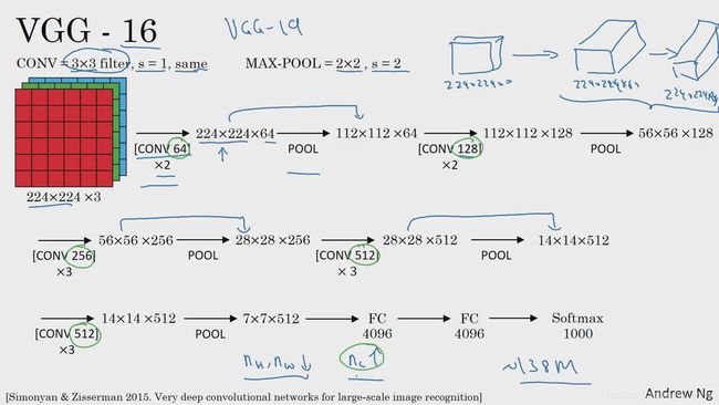
3.VGG-16
https://arxiv.org/pdf/1409.1556.pdf
VGG网络没那么多超参数,这是一种只需要专注于构建卷积层的简单网络,
包含1.38亿个参数,即使现在看也是非常庞大的网络,但是其结构并不复杂,这点很吸引人,并且这种网络结构很规整,都是几个卷积层后面跟着可以压缩的池化层,同时卷积层的过滤器数量变化存在一定的规律。
正是这种设计网络结构的简单规则,相对一致的网路结构对研究者很有吸引力。
它的主要缺点,需要训练的特征数量非常巨大。
有些文章还介绍了VGG-19,它比VGG-16还大,由于VGG-16和VGG-19表现几乎不分高下,所以很多人还是会使用VGG-16;
另一点,随着网络的加深,图像的高度和宽度都在以一定规律缩小,而信道在不断增加。且这个变化是有规律的。从这点看,这篇论文很吸引人。
阅读论文,**建议从AlexNet开始,VGG, LeNet-5,**虽然有些难懂,但对于了解这些网络结构很有帮助
LeNet Lab
这是以前上优达学成无人驾驶课的一个小实验,LeNet在手写体mnist数据集的实现
Load Data
Load the MNIST data, which comes pre-loaded with TensorFlow.
You do not need to modify this section.
读取TensorFlow中自带的Mnist数据集
from tensorflow.examples.tutorials.mnist import input_data

mnist = input_data.read_data_sets("MNIST_data/", reshape=False)
X_train, y_train           = mnist.train.images, mnist.train.labels
X_validation, y_validation = mnist.validation.images, mnist.validation.labels
X_test, y_test             = mnist.test.images, mnist.test.labels

assert(len(X_train) == len(y_train))
assert(len(X_validation) == len(y_validation))
assert(len(X_test) == len(y_test))

print()
print("Image Shape: {}".format(X_train[0].shape))
print()
print("Training Set:   {} samples".format(len(X_train)))
print("Validation Set: {} samples".format(len(X_validation)))
print("Test Set:       {} samples".format(len(X_test)))
Extracting MNIST_data/train-images-idx3-ubyte.gz
Extracting MNIST_data/train-labels-idx1-ubyte.gz
Extracting MNIST_data/t10k-images-idx3-ubyte.gz
Extracting MNIST_data/t10k-labels-idx1-ubyte.gz

Image Shape: (28, 28, 1)

Training Set:   55000 samples
Validation Set: 5000 samples
Test Set:       10000 samples
The MNIST data that TensorFlow pre-loads comes as 28x28x1 images.
However, the LeNet architecture only accepts 32x32xC images, where C is the number of color channels.
In order to reformat the MNIST data into a shape that LeNet will accept, we pad the data with two rows of zeros on the top and bottom, and two columns of zeros on the left and right (28+2+2 = 32).
You do not need to modify this section.
将数据扩展为LeNet可处理的32x32x1格式
import numpy as np

# Pad images with 0s
X_train      = np.pad(X_train, ((0,0),(2,2),(2,2),(0,0)), 'constant')
X_validation = np.pad(X_validation, ((0,0),(2,2),(2,2),(0,0)), 'constant')
X_test       = np.pad(X_test, ((0,0),(2,2),(2,2),(0,0)), 'constant')

print("Updated Image Shape: {}".format(X_train[0].shape))
#print(X_train[0])
Updated Image Shape: (32, 32, 1)
Visualize Data
View a sample from the dataset.
You do not need to modify this section.
import random
import numpy as np
import matplotlib.pyplot as plt
%matplotlib inline

index = random.randint(0, len(X_train))
image = X_train[index].squeeze()

plt.figure(figsize=(1,1))
plt.imshow(image, cmap="gray")
print(y_train[index])
9
Preprocess Data
Shuffle the training data. 数据随机打散,清洗数据
You do not need to modify this section.
from sklearn.utils import shuffle

X_train, y_train = shuffle(X_train, y_train)
Setup TensorFlow
The EPOCH and BATCH_SIZE values affect the training speed and model accuracy.
You do not need to modify this section.
import tensorflow as tf

EPOCHS = 5
BATCH_SIZE = 128
Visualizing Layers
# image_input: the test image being fed into the network to produce the feature maps
# tf_activation: should be a tf variable name used during your training procedure that represents the calculated state of a specific weight layer
# Note: that to get access to tf_activation, the session should be interactive which can be achieved with the following commands.
# sess = tf.InteractiveSession()
# sess.as_default()

# activation_min/max: can be used to view the activation contrast in more detail, by default matplot sets min and max to the actual min and    max values of the output
# plt_num: used to plot out multiple different weight feature map sets on the same block, just extend the plt number for each new feature map entry

def outputFeatureMap(image_input, tf_activation, activation_min=-1, activation_max=-1 ,plt_num=1):
    # Here make sure to preprocess your image_input in a way your network expects
    # with size, normalization, ect if needed
    # image_input =
    # Note: x should be the same name as your network's tensorflow data placeholder variable
    # If you get an error tf_activation is not defined it maybe having trouble accessing the variable from inside a function
    activation = tf_activation.eval(session=sess,feed_dict={
     x : image_input})
    featuremaps = activation.shape[3]
    plt.figure(plt_num, figsize=(15,15))
    for featuremap in range(featuremaps):
        plt.subplot(6,8, featuremap+1) # sets the number of feature maps to show on each row and column
        plt.title('FeatureMap ' + str(featuremap)) # displays the feature map number
        if activation_min != -1 & activation_max != -1:
            plt.imshow(activation[0,:,:, featuremap], interpolation="nearest", vmin =activation_min, vmax=activation_max, cmap="gray")
        elif activation_max != -1:
            plt.imshow(activation[0,:,:, featuremap], interpolation="nearest", vmax=activation_max, cmap="gray")
        elif activation_min !=-1:
            plt.imshow(activation[0,:,:, featuremap], interpolation="nearest", vmin=activation_min, cmap="gray")
        else:
            plt.imshow(activation[0,:,:, featuremap], interpolation="nearest", cmap="gray")
TODO: Implement LeNet-5
Implement the LeNet-5 neural network architecture.
This is the only cell you need to edit.
Input
The LeNet architecture accepts a 32x32xC image as input, where C is the number of color channels. Since MNIST images are grayscale, C is 1 in this case.
Architecture
Layer 1: Convolutional. The output shape should be 28x28x6.
Activation. Your choice of activation function.
Pooling. The output shape should be 14x14x6.
Layer 2: Convolutional. The output shape should be 10x10x16.
Activation. Your choice of activation function.
Pooling. The output shape should be 5x5x16.
Flatten. Flatten the output shape of the final pooling layer such that it’s 1D instead of 3D. The easiest way to do is by using tf.contrib.layers.flatten, which is already imported for you.
Layer 3: Fully Connected. This should have 120 outputs.
Activation. Your choice of activation function.
Layer 4: Fully Connected. This should have 84 outputs.
Activation. Your choice of activation function.
Layer 5: Fully Connected (Logits). This should have 10 outputs.
Output
Return the result of the 3nd fully connected layer.
Design model architecture
final model architecture looks like below, consisted of the following layers:
| Layer | Description |
|---|---|
| Input | 32x32x1 RGB image |
| Convolution 5x5x1 | 1x1 stride, valid padding,outputs 28x28x6 |
| RELU | |
| Max pooling | 2x2 stride, outputs 14x14x6 |
| Convolution 5x5x6 | 1x1 stride, valid padding, outputs 10x10x16 |
| RELU | |
| Max pooling | 2x2 stride, outputs 5x5x16 |
| RELU | |
| Flatten | input 5x5x16, outputs 400 |
| Fully connected | intputs 400, outputs 120 |
| RELU | |
| Fully connected | intputs 120, outputs 84 |
| RELU | |
| Fully connected | inputs 84, outputs 10 |
| Softmax | 10x1 |
from tensorflow.contrib.layers import flatten

def LeNet(x):
    # Arguments used for tf.truncated_normal, randomly defines variables for the weights and biases for each layer
    mu = 0
    sigma = 0.1

    # TODO: Layer 1: Convolutional. Input = 32x32x1. Output = 28x28x6.
    conv1_W = tf.Variable(tf.truncated_normal((5,5,1,6),mean=mu, stddev=sigma))
    conv1_b = tf.Variable(tf.zeros(6))
    conv1 = tf.nn.conv2d(x,conv1_W,strides=[1,1,1,1],padding='VALID') + conv1_b #(32-5+1)/1=28  28x28x6

    # TODO: Activation.
    conv1 = tf.nn.relu(conv1)

    # TODO: Pooling. Input = 28x28x6. Output = 14x14x6.
    conv1 = tf.nn.max_pool(conv1,ksize=[1,2,2,1],strides=[1,2,2,1],padding='VALID')

    # TODO: Layer 2: Convolutional. Output = 10x10x16.
    #input:14x14x6
    conv2_W = tf.Variable(tf.truncated_normal((5,5,6,16),mean=mu, stddev=sigma))
    conv2_b = tf.Variable(tf.zeros(16))
    conv2 = tf.nn.conv2d(conv1,conv2_W,strides=[1,1,1,1],padding='VALID') + conv2_b #(14-5+1)/1=10  10x10x16

    # TODO: Activation.
    conv2 = tf.nn.relu(conv2)

    # TODO: Pooling. Input = 10x10x16. Output = 5x5x16.
    conv2 = tf.nn.max_pool(conv2,ksize=[1,2,2,1],strides=[1,2,2,1],padding='VALID')

    # TODO: Flatten. Input = 5x5x16. Output = 400.
    fc0 = flatten(conv2)

    # TODO: Layer 3: Fully Connected. Input = 400. Output = 120.
    fc1_W = tf.Variable(tf.truncated_normal((400,120),mean=mu, stddev=sigma))
    fc1_b = tf.Variable(tf.zeros(120))
    fc1 = tf.matmul(fc0,fc1_W) + fc1_b

    # TODO: Activation.
    fc1 = tf.nn.relu(fc1)

    # TODO: Layer 4: Fully Connected. Input = 120. Output = 84.
    fc2_W = tf.Variable(tf.truncated_normal((120,84),mean=mu, stddev=sigma))
    fc2_b = tf.Variable(tf.zeros(84))
    fc2 = tf.matmul(fc1,fc2_W) + fc2_b
    # TODO: Activation.
    fc2 = tf.nn.relu(fc2)

    # TODO: Layer 5: Fully Connected. Input = 84. Output = 10.
    fc3_W = tf.Variable(tf.truncated_normal((84,10),mean=mu, stddev=sigma))
    fc3_b = tf.Variable(tf.zeros(10))
    logits = tf.matmul(fc2,fc3_W) + fc3_b
    print("---logits type:",type(logits))
    return logits
Features and Labels
Train LeNet to classify MNIST data.
x is a placeholder for a batch of input images.
y is a placeholder for a batch of output labels.
You do not need to modify this section.
x = tf.placeholder(tf.float32, (None, 32, 32, 1))
y = tf.placeholder(tf.int32, (None))
one_hot_y = tf.one_hot(y, 10)
print(one_hot_y)
print("one_hot_y type:",type(one_hot_y))
Tensor("one_hot_1:0", dtype=float32)
one_hot_y type:
Training Pipeline
Create a training pipeline that uses the model to classify MNIST data.
You do not need to modify this section.
rate = 0.001

logits = LeNet(x)
cross_entropy = tf.nn.softmax_cross_entropy_with_logits(labels=one_hot_y, logits=logits)
loss_operation = tf.reduce_mean(cross_entropy)
optimizer = tf.train.AdamOptimizer(learning_rate = rate)
training_operation = optimizer.minimize(loss_operation)
Model Evaluation
Evaluate how well the loss and accuracy of the model for a given dataset.
You do not need to modify this section.
correct_prediction = tf.equal(tf.argmax(logits, 1), tf.argmax(one_hot_y, 1))
accuracy_operation = tf.reduce_mean(tf.cast(correct_prediction, tf.float32))


def evaluate(X_data, y_data):
    num_examples = len(X_data)
    total_accuracy = 0 #统计正确预测总个数
    sess = tf.get_default_session()
    for offset in range(0, num_examples, BATCH_SIZE):
        batch_x, batch_y = X_data[offset:offset+BATCH_SIZE], y_data[offset:offset+BATCH_SIZE]
        accuracy = sess.run(accuracy_operation, feed_dict={
     x: batch_x, y: batch_y})
        #print("accuracy:",accuracy) #返回本批次的准确率
        total_accuracy += (accuracy * len(batch_x)) #
        #print("accuracy:{},total_accuracy:{}".format(accuracy,total_accuracy))

    return total_accuracy / num_examples
Train the Model
Run the training data through the training pipeline to train the model.
Before each epoch, shuffle the training set.
After each epoch, measure the loss and accuracy of the validation set.
Save the model after training.
You do not need to modify this section.
saver = tf.train.Saver()
with tf.Session() as sess:
    sess.run(tf.global_variables_initializer())
    num_examples = len(X_train)

    print("Training...")
    print()
    for i in range(EPOCHS):
        X_train, y_train = shuffle(X_train, y_train)
        for offset in range(0, num_examples, BATCH_SIZE):
            end = offset + BATCH_SIZE
            batch_x, batch_y = X_train[offset:end], y_train[offset:end]
            sess.run(training_operation, feed_dict={
     x: batch_x, y: batch_y})

        validation_accuracy = evaluate(X_validation, y_validation)
        print("EPOCH {} ...".format(i+1))
        print("Validation Accuracy = {:.3f}".format(validation_accuracy))
        print()


    saver.save(sess, './lenet')
    print("Model saved")
Training...

EPOCH 1 ...
Validation Accuracy = 0.969

EPOCH 2 ...
Validation Accuracy = 0.979

EPOCH 3 ...
Validation Accuracy = 0.983

EPOCH 4 ...
Validation Accuracy = 0.985

EPOCH 5 ...
Validation Accuracy = 0.983

Model saved
Evaluate the Model
Once you are completely satisfied with your model, evaluate the performance of the model on the test set.
Be sure to only do this once!
If you were to measure the performance of your trained model on the test set, then improve your model, and then measure the performance of your model on the test set again, that would invalidate your test results. You wouldn’t get a true measure of how well your model would perform against real data.
You do not need to modify this section.
with tf.Session() as sess:
    saver.restore(sess, tf.train.latest_checkpoint('.'))

    test_accuracy = evaluate(X_test, y_test)
    print("Test Accuracy = {:.3f}".format(test_accuracy))
INFO:tensorflow:Restoring parameters from ./lenet
Test Accuracy = 0.985


