吴恩达机器学习作业4---Neural Networks Learning

Neural Networks Learning

代码分析

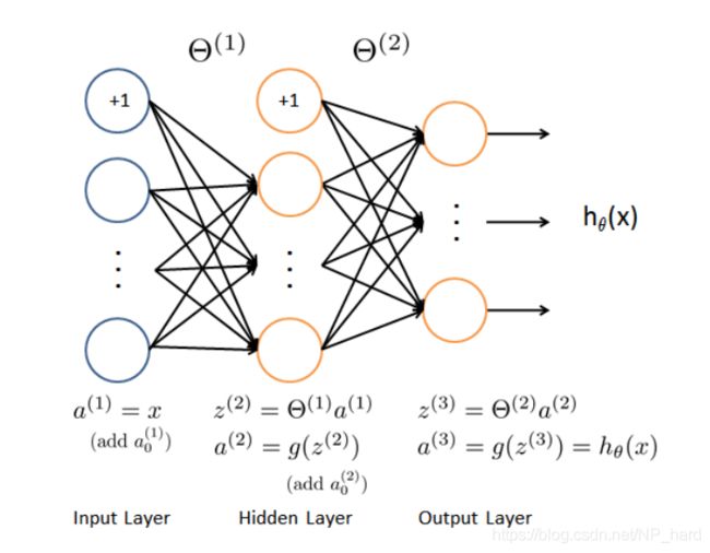
首先，下图为本次需要构建的神经网络模型

输入为一张20x20的图片，用以识别手写数字

该神经网络分为三层，输入层有400+1（bias unit）个单元，隐藏层有25+1个单元，输出层有10个单元

训练一个神经网络模型主要分为几个步骤

1. 随机初始化参数θ
2. 执行正向传播，得到每一层的（z，a）
3. 执行反向传播，对参数进行梯度下降

为了构建神经网络模型，我们需要实现正向传播函数，cost值计算函数，反向传播函数，由这三个函数来对参数theta进行优化，最终得到cost值最小的模型

首先，导入所需的类库

import numpy as np
import matplotlib.pyplot as plt
import pandas as pd
import scipy.io #Used to load the OCTAVE *.mat files
import scipy.misc #Used to show matrix as an image
import matplotlib.cm as cm #Used to display images in a specific colormap
import random #To pick random images to display
import scipy.optimize #fmin_cg to train neural network
import itertools
from scipy.special import expit #Vectorized sigmoid function

%matplotlib inline

导入数据

这次作业提供了已经优化好的参数theta以供测试

#导入已经优化后的单隐藏层神经网络的参数theta
datafile = 'data/ex3weights.mat'
mat = scipy.io.loadmat( datafile )
Theta1, Theta2 = mat['Theta1'], mat['Theta2']
# Theta1 has size 25 x 401
# Theta2 has size 10 x 26

还有一些全局变量

input_layer_size = 400
hidden_layer_size = 25
output_layer_size = 10 
n_training_samples = X.shape[0]

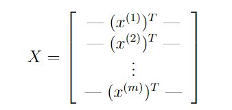
好了，现在开始导入训练集

X是5000张图片的矩阵，y是每张图片的数字类别

#导入数据，由于ex3和ex4的数据相同，这里导入ex3的数据
datafile = 'data/ex3data1.mat'
mat = scipy.io.loadmat( datafile )

X, y = mat['X'], mat['y']

#在X矩阵前插入全为1的一列作为bias unit
X = np.insert(X,0,1,axis=1)
#测试
print ("'y' shape: %s. Unique elements in y: %s"%(mat['y'].shape,np.unique(mat['y'])))
print ("'X' shape: %s. X[0] shape: %s"%(X.shape,X[0].shape))

#X is 5000 images. Each image is a row. Each image has 400 pixels unrolled (20x20)
#y is a classification for each image. 1-10, where "10" is the handwritten "0"

测试结果

'y' shape: (5000, 1). Unique elements in y: [ 1  2  3  4  5  6  7  8  9 10]
'X' shape: (5000, 401). X[0] shape: (401,)

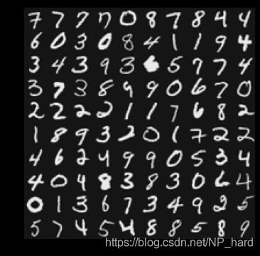
可视化这些数据

将400的行向量转为20x20的ndarray的函数

def getDatumImg(row):
    width, height = 20, 20
    #row.shape=401
    #将400的行向量转为20x20的narray
    square = row[1:].reshape(width,height)
    return square.T

可视化数据为黑白图片

def displayData(X,indices_to_display = None):
    #图片格式为20x20
    width, height = 20, 20
    #10x10的图像网格
    nrows, ncols = 10, 10
    #5000张图片中随机抽取100张
    if not indices_to_display:
        indices_to_display = random.sample(range(X.shape[0]), nrows*ncols)
    #200x200的narray
    big_picture = np.zeros((height*nrows,width*ncols))
    #遍历图片集,为空白的大图片赋值
    irow, icol = 0, 0
    for idx in indices_to_display:
        if icol == ncols:
            irow += 1
            icol  = 0
        iimg = getDatumImg(X[idx])
        #将这块区域的图片赋值
        big_picture[irow*height:irow*height+iimg.shape[0],icol*width:icol*width+iimg.shape[1]] = iimg
        icol += 1
    #输出图片
    fig = plt.figure(figsize=(6,6))
    plt.imshow(big_picture,cmap ='gray')

测试

在正式对神经网络模型进行训练前，我们需要对数据进行处理

对于本次作业而言，参数theta为矩阵，不利于进行计算，这里我们要将其展开为行向量

该函数将theta_list展开为一个（n，1）行向量ndarray

#将theta_list展开为一个（n，1）行向量ndarray
def flattenParams(thetas_list):
    #将参数θ矩阵展开为行向量并合并到一个list中
    flattened_list = [ mytheta.flatten() for mytheta in thetas_list ]
    #将装有两个ndarray的list转换为一个list
    combined = list(itertools.chain.from_iterable(flattened_list))
    assert len(combined) == (input_layer_size+1)*hidden_layer_size + \
                            (hidden_layer_size+1)*output_layer_size
    return np.array(combined).reshape((len(combined),1))

该函数将行向量ndarray重新展开为参数矩阵

#将行向量ndarray重新展开为参数矩阵
def reshapeParams(flattened_array):
    theta1 = flattened_array[:(input_layer_size+1)*hidden_layer_size].reshape((hidden_layer_size,input_layer_size+1))
    theta2 = flattened_array[(input_layer_size+1)*hidden_layer_size:].reshape((output_layer_size,hidden_layer_size+1))
    return [ theta1, theta2 ]

下面这两个函数可以对X进行展开与收缩

def flattenX(myX):
    return np.array(myX.flatten()).reshape((n_training_samples*(input_layer_size+1),1))

def reshapeX(flattenedX):
    return np.array(flattenedX).reshape((n_training_samples,input_layer_size+1))

好了，下面开始编写正向传播算法和cost值计算函数

下面的函数为正向传播函数，参数为一张图片和初始化的theta
它将会计算每一层的（z，a）

#参数为训练集的某个数据，每层神经网络的参数theta
def propagateForward(row,Thetas):
    features = row#row为某个训练集
    zs_as_per_layer = []
    #遍历每一层
    for i in range(len(Thetas)):  
        Theta = Thetas[i]
        z = Theta.dot(features).reshape((Theta.shape[0],1))
        a = expit(z)
        zs_as_per_layer.append( (z, a) )
        if i == len(Thetas)-1:
            return np.array(zs_as_per_layer)
        a = np.insert(a,0,1) #加上bias unit
        features = a

下面的函数为cost值计算函数，它将会计算所有训练集的平均cost值

#传入处理过的参数theta，数据集（X，y）
def computeCost(mythetas_flattened,myX_flattened,myy,mylambda=0.):
    #先将参数重新变为矩阵
    mythetas = reshapeParams(mythetas_flattened)
    myX = reshapeX(myX_flattened)
    total_cost = 0.
    m = n_training_samples
    #先使用遍历训练集的方法，后续会考虑向量化
    for irow in range(m):
        myrow = myX[irow]#某个图片
        myhs = propagateForward(myrow,mythetas)[-1][1]#myhs是神经网络输出层的激发值
        tmpy  = np.zeros((10,1))#tmpy为某个图像数字的向量值
        tmpy[myy[irow]-1] = 1
        #计算cost值
        mycost = -tmpy.T.dot(np.log(myhs))-(1-tmpy.T).dot(np.log(1-myhs))
        total_cost += mycost
    total_cost = float(total_cost) / m
    # 计算正则项
    total_reg = 0.
    for mytheta in mythetas:
        total_reg += np.sum(mytheta*mytheta) #element-wise multiplication
    total_reg *= float(mylambda)/(2*m)
    return total_cost + total_reg

我们测试一下训练好的参数theta的平均cost如何

#you should see that the cost is about 0.287629
myThetas = [ Theta1, Theta2 ]
#测试
print (computeCost(flattenParams(myThetas),flattenX(X),y))

输出：0.28762916516131876

下面我们测试一下加入正则化项的平均cost如何

#and lambda = 1, you should see that the cost is about 0.383770
myThetas = [ Theta1, Theta2 ]
print (computeCost(flattenParams(myThetas),flattenX(X),y,mylambda=1.))

输出：0.3844877962428938

明显看出加入正则化项之后的cost要大，即参数对训练集的拟合度减小，防止过拟合

好，下面进行反向传播算法的编写

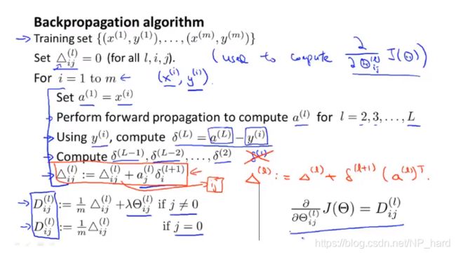
就像对其他模型进行梯度下降算法，我们需要得到J(θ)对θ的偏导数才能进行
梯度下降
$${\theta }_{ij}:={\theta }_{ij}-\alpha \frac{\partial J(\theta )}{\partial {\theta }_{ij}^{(l)}}$$

而通过数学证明（忽略α）
$$\frac{\partial J(\theta )}{\partial {\theta }_{ij}^{(l)}}=a_j^{(l)}{\delta }_i^{(l+1)}$$
又因为某个单元的梯度为所有训练集的平均梯度

故
$$\frac{\partial J(\theta )}{\partial {\theta }_{ij}^{(l)}}=\frac{1}{m}{\Delta }_{ij}^{(l)}$$

这是反向传播算法的函数，返回D1，D2展开的numpy数组

#传入处理过的参数theta，数据集（X，y）
#返回每层参数theta的偏导数
def backPropagate(mythetas_flattened,myX_flattened,myy,mylambda=0.):
    
    #首先将行向量转化为矩阵
    mythetas = reshapeParams(mythetas_flattened)
    myX = reshapeX(myX_flattened)

    #Note: the Delta matrices should include the bias unit
    #The Delta matrices have the same shape as the theta matrices
    #初始化δ
    Delta1 = np.zeros((hidden_layer_size,input_layer_size+1))
    Delta2 = np.zeros((output_layer_size,hidden_layer_size+1))

    # Loop over the training points (rows in myX, already contain bias unit)
    m = n_training_samples
    for irow in range(m):
        myrow = myX[irow]#某个图像
        a1 = myrow.reshape((input_layer_size+1,1))#再次将图像矩阵展开为行向量
        # propagateForward returns (zs, activations) for each layer excluding the input layer
        #temp包含除了输入层的（z，a）
        temp = propagateForward(myrow,mythetas)
        z2 = temp[0][0]
        a2 = temp[0][1]
        z3 = temp[1][0]
        a3 = temp[1][1]
        
        tmpy = np.zeros((10,1))#tmpy为某个图像数字的向量值（即答案）
        tmpy[myy[irow]-1] = 1
        
        delta3 = a3 - tmpy 
        delta2 = mythetas[1].T[1:,:].dot(delta3)*sigmoidGradient(z2) #参数θ忽略bias unit
        a2 = np.insert(a2,0,1,axis=0)
        Delta1 += delta2.dot(a1.T) #(25,1)x(1,401) = (25,401) (correct)
        Delta2 += delta3.dot(a2.T) #(10,1)x(1,25) = (10,25) (should be 10,26)
        
    D1 = Delta1/float(m)
    D2 = Delta2/float(m)
    
    #正则化
    D1[:,1:] = D1[:,1:] + (float(mylambda)/m)*mythetas[0][:,1:]
    D2[:,1:] = D2[:,1:] + (float(mylambda)/m)*mythetas[1][:,1:]
    
    return flattenParams([D1, D2]).flatten()

利用提供的参数theta计算一次梯度

#Actually compute D matrices for the Thetas provided
flattenedD1D2 = backPropagate(flattenParams(myThetas),flattenX(X),y,mylambda=0.)
D1, D2 = reshapeParams(flattenedD1D2)

检查反向传播计算的梯度是否准确

#传入参数，偏导数，数据集（X，y）
def checkGradient(mythetas,myDs,myX,myy,mylambda=0.):
    myeps = 0.0001
    #将参数化为行向量
    flattened = flattenParams(mythetas)
    flattenedDs = flattenParams(myDs)
    myX_flattened = flattenX(myX)
    n_elems = len(flattened) 
    
    #Pick ten random elements, compute numerical gradient, compare to respective D's
    #随机选择10个元素，计算偏导数以比较
    for i in range(10):
        x = int(np.random.rand()*n_elems)
        epsvec = np.zeros((n_elems,1))
        epsvec[x] = myeps
        cost_high = computeCost(flattened + epsvec,myX_flattened,myy,mylambda)
        cost_low  = computeCost(flattened - epsvec,myX_flattened,myy,mylambda)
        mygrad = (cost_high - cost_low) / float(2*myeps)
        print ("Element: %d. Numerical Gradient = %f. BackProp Gradient = %f."%(x,mygrad,flattenedDs[x]))

测试

checkGradient(myThetas,[D1, D2],X,y)

Element: 10113. Numerical Gradient = -0.000927. BackProp Gradient = -0.000927.
Element: 3468. Numerical Gradient = -0.000036. BackProp Gradient = -0.000036.
Element: 4309. Numerical Gradient = 0.000051. BackProp Gradient = 0.000051.
Element: 9991. Numerical Gradient = -0.000149. BackProp Gradient = -0.000149.
Element: 1241. Numerical Gradient = 0.000001. BackProp Gradient = 0.000001.
Element: 9973. Numerical Gradient = 0.000174. BackProp Gradient = 0.000174.
Element: 8678. Numerical Gradient = 0.000160. BackProp Gradient = 0.000160.
Element: 4224. Numerical Gradient = -0.000084. BackProp Gradient = -0.000084.
Element: 526. Numerical Gradient = -0.000085. BackProp Gradient = -0.000085.
Element: 7040. Numerical Gradient = 0.000085. BackProp Gradient = 0.000085.

好的，算法都编写完了，我们开始自己优化参数theta吧

该函数可以计算得出优化后的θ

#训练神经网络模型
def trainNN(mylambda=0.):
    #随机初始化theta
    randomThetas_unrolled = flattenParams(genRandThetas())
    #优化theta，参数为：代价函数，初始参数theta，数据集（X，y）
    result = scipy.optimize.fmin_cg(computeCost, x0=randomThetas_unrolled, fprime=backPropagate, \
                               args=(flattenX(X),y,mylambda),maxiter=50,disp=True,full_output=True)
    return reshapeParams(result[0])

测试

learned_Thetas = trainNN()

Current function value: 0.252900
Iterations: 50
Function evaluations: 115
Gradient evaluations: 115

下面计算模型在训练集的准确率

这个函数可以返回概率最大的数字

#返回概率最大的数字
def predictNN(row,Thetas):
    classes = list(range(1,10)) + [10]
    output = propagateForward(row,Thetas)
    #-1 means last layer, 1 means "a" instead of "z"
    return classes[np.argmax(output[-1][1])]

这个函数计算模型准确率

#计算模型准确率
def computeAccuracy(myX,myThetas,myy):
    n_correct, n_total = 0, myX.shape[0]
    for irow in range(n_total):
        if int(predictNN(myX[irow],myThetas)) == int(myy[irow]): 
            n_correct += 1
    print ("Training set accuracy: %0.1f%%"%(100*(float(n_correct)/n_total)))

测试

computeAccuracy(X,learned_Thetas,y)

Training set accuracy: 97.0%

看看正则化参数为10时的准确率

#Let's see if I set lambda to 10, if I get the same thing
learned_regularized_Thetas = trainNN(mylambda=10.)

Current function value: 1.071414
Iterations: 49
Function evaluations: 164
Gradient evaluations: 152

computeAccuracy(X,learned_regularized_Thetas,y)

Training set accuracy: 93.6%

可以看出正则化的效果

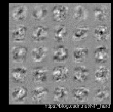
可视化隐藏层所识别的图像

def displayHiddenLayer(myTheta):
    """
    Function that takes slices of the first Theta matrix (that goes from
    the input layer to the hidden layer), removes the bias unit, and reshapes
    it into a 20x20 image, and shows it
    """
    #删去bias unit:
    myTheta = myTheta[:,1:]
    assert myTheta.shape == (25,400)
    
    width, height = 20, 20
    nrows, ncols = 5, 5
        
    big_picture = np.zeros((height*nrows,width*ncols))
    
    irow, icol = 0, 0
    for row in myTheta:
        if icol == ncols:
            irow += 1
            icol  = 0
        #add bias unit back in?
        iimg = getDatumImg(np.insert(row,0,1))#将400的行向量转为20x20的ndarray
        big_picture[irow*height:irow*height+iimg.shape[0],icol*width:icol*width+iimg.shape[1]] = iimg
        icol += 1
    fig = plt.figure(figsize=(6,6))
    plt.imshow(big_picture,cmap ='gray')

测试

displayHiddenLayer(learned_Thetas[0])

数据集

可以上kaggle搜索这些数据

ex4data1.mat

ex4weights.mat