Regularization & Dimension reduction

这周简直要忙疯，但是感觉这个seminar的课真的是对一个初学者的自己很有帮助，了解了很多SL的算法和基本知识，既然做了，就分享下regularization这部分的笔记吧~
内容整合了ISL("An Introduction to Statistical Learning" by James, Witten, Hastie and Tibshirani)和ESL(The Elements of Statistical Learning:Data Mining, Inference, and Prediction by Hastie, Tibshirani and Friedman)两本书

Useful R packages:
Glmnet
ElasticNet
eNetXplorer (后附简单的running example，强推（带强烈的个人感情色彩）其实没什么特别的，但是脑残粉就是喜欢哈哈哈orz）

Shrinkage/Regularization

• A technique constrains/regularizes/shrinks the coefficient estimates, more continuous, could also performs variable selection.
• Fitting a model involving all p predictors. However, the estimated coefficients are shrunken towards zero relative to the least squares estimates.

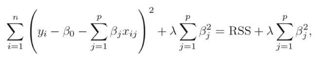
Ridge Regression

Ridge coefficient estimates = argmin{RSS+shrinkage penalty} (L2 panelty)
The idea of penalizing by the sum-of-squares of the parameters is also used in neural networks, where it is known as weight decay.

or another expression

• Shrinkage penalty is small when s are close to zero, so has the effect of shrinking the estimates of to zero.
• is important: = 0, the penalty has no effect; grows, panelty grows, and the coefficients approach zero.
• Cross-validation could be used to choose .
• Not equivariant underscaling of inputs, apply after standardizing the predictors.

---

Ridge regression bias-variance trade-off, compared with least squares.

• increases, the flexibility decreases, leading to decreased variance but increased bias.
• p~n/ p>n ridge regression could out perform well by trading off a small increase in bias for a large decrease in variance.
• Substantial computational advantage compared with best subset selection.

Disadvantage:
Unlike best subset, forward stepwise, and backward stepwise selection, which will generally select models that involve just a subset of the variables, ridge regression will include all p predictors in the final model(unless = ) -- a challenge in model interpretation esp p is large.

Lasso

Lasso coefficient estimates = argmin{RSS+L1 penalty}

or another expression

• Also shrinks the coefficient estimates to zero.
• L1 penalty has the effect of forcing some of the coefficient estimates = 0 when is sufficiently large. So, Lasso also performs variable selection.
• Much easier to interperet than Ridge regression.

The limitations of the lasso

• If p>n, the lasso selects at most n variables. The number of selected predictors is bounded by the number of samples.
• Grouped variables: the lasso fails to do grouped selection. It tends to select one variable from a group and ignore the others.

不得不提一下现在应用更广泛的Elastic Net

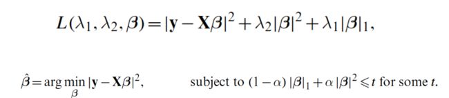
Elastic Net

Reference paper: Zou, H., & Hastie, T. (2005). Regularization and variable selection via the elastic net. Journal of the Royal Statistical Society: Series B (Statistical Methodology), 67(2), 301-320.

Elastic Net coefficient estimates = argmin{RSS+elastic net penalty}
elastic net penalty -- a convex combination of the lasso and ridge penalty. When α = 1, the naive elastic net becomes simple ridge regression. (opposite to the α of glmnet package)

• The L1 part of the penalty generates a sparse model.
• The quadratic part of the penalty:
  -- Removes the limitation on the number of selected variables
  -- Encourages grouping effect;
  -- Stabilizes the L1 regularization path

Comparing the Lasso, Ridge and ElasticNet

• why is it that Lasso, unlike ridge, results in coefficient estimates that are exactly to zero?

  
  
  

• Lasso, Ridge and Elastic Net
  useful simulations with R: https://www4.stat.ncsu.edu/~post/josh/LASSO_Ridge_Elastic_Net_-_Examples.html

• 1.e.g.1: Small signal, lots of noise, unrelated predictors. -- Lasso is the winner!
  

  2. e.g.2: Big signal, big noise, unrelated predictors.-- Ridge is the winner!
     

  3. e.g.3: Varying signals. High correlation between predictors -- Elastic Net is the winner! (the best solution is “close” to Ridge, but Ridge in fact performs the worst.)
     

• In general, one might expect the lasso to perform better in a setting where a relatively small number of predictors have substantial coefficients, and the remaining predictors have coefficients that are very small or that equal zero. Ridge regression will perform better when the response is a function of many predictors, all with coefficients of roughly equal size.

• However, the number of predictors that is related to the response is never known a priori for real data sets. Cross-validation!

• Selecting the Tuning Parameter: Cross-validation!

Dimension Reduction

• Approaches that transform the predictors and then fit a least squares model using the transformed variables.
• 2 steps: 1-choose transformed predictors Z1, Z2,...ZM; 2-The model is fit using these M predictors.
• 2 appaches covered to choose M predictors: PCR and PLS

PCR (Principal Components Regression)

• Z1, Z2,...ZM as principal components, capture the M most the information contained in the predictors

approach:

1. Constructing the first M principal components -- typically chosen by cross-validation
2. Using the predictors in a linear regression model that is fit using least squares.

• Pros: performs well when the first few principal components are sufficient to capture most of the variation in the predictors as well as the relationship with the response.

• Cons: - doesn't perform well when many principal componets are required in order to adequately model the response.

  ​ - It is not a feature selection method since M components used is a linear combination of all p of the original features. Still hard to interpret?

PLS (Partial Least Squares)

• A supervised alternative to PCR
• Construct M features in a supervised way -- make the use of response Y in order to identify new features related to the response (find directions explain both response and predictors).
• PLS places the highest weight on the variables that are most strongly related to the response.

A Comparison of the Selection and Shrinkage Methods

Book ESL: 3.6 p82

correlation between X1 and X2 = 0.5

• PLS, PCR and ridge regression tend to behave similarly. Ridge regression may be preferred because it shrinks smoothly, rather than in discrete steps.
• Lasso falls somewhere between ridge regression and best subset regression, and enjoys some of the properties of each.

Tips: high dimensional data

• highly easy to get overfiting of the data
• Be careful to interpret the results: just one of many possible models for the prediction.
• Be careful in reporting errors and measures: report results on an independent test set or cross-validation errors instead of training set.

Simple R example on ElasticNet

• 先看看内置的测试数据长什么样
  Test data: H1N1_Flow.
  Data from a cohort of healthy subjects vaccinated against influenza virus H1N1. Cell population frequencies from deep-phenotyping flow cytometry were determined longitudinally.

# install.packages(eNetXplorer)
library(eNetXplorer)
data("H1N1_Flow")
H1N1_Flow$predictor_day7[1:3,1:12]

• 非常好用的一步，省了好多coding的活，直接替你做了crosss-validation，找到最合适的值（此处与glmnet定义的相同，与original Elastic Net paper相反）
  Linear models of using day7 cell population data to predict day70 H1N1 serum titers:
  Using eNetXplorer, a family of elastic net models is generated from ridge (a = 0) to lasso (a = 1). For each a, the choice of a is guided by cross-validation.

fit <- eNetXplorer(x=H1N1_Flow$predictor_day7, y=H1N1_Flow$response_numer[rownames(
H1N1_Flow$predictor_day7)], family="gaussian", n_run=25, n_perm_null=15)

还显示进度哦

GLM的family现在还支持two-class logistic和multinomial regression，以后的版本会更新Poisson regression and the Cox model for survival data.

• Why penalty parameter is selected? Given alpha, quality function across (User-defined QFs can be provided)

plot(fit, plot.type="lambdaVsQF", alpha.index=4)

• Summary plots to display the performance of all models in the elastic net family with different a. (各个plot都集中在一个方程中，很好用）

plot(fit, plot.type = "summary")

• 迅速找到关键因子：
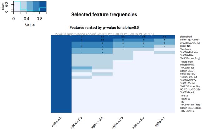
  A heatmap plot of feature statistics across a, which includes statistical significance annotations for individual features.
  The frequencies of each feature was chosen to be included in each model over the entire elastic net family(a=[0,1]). As a increases, we could observe the emergence of several significant features. As lasso is approached, only the top few features remain.

plot(fit, plot.type = "featureHeatmap", stat="freq", alpha.index=4)

参考文献：
https://www.biorxiv.org/content/early/2018/04/30/305870