【Python计算机视觉】图像拼割、创建全景图像
目录
- 一、引入
-
- 1.1 特征匹配
- 1.2 问题:Bad Example
-
- 1.2.1 “鬼影”
- 1.2.2 错误匹配的干扰
- 1.3 解决:Simple Example
-
- 1.3.1 拟合消除噪声点
- 1.3.2 参数求解:RAndom SAmple Consensus
- 1.3.3 APAP算法
- 1.3.4 寻找最佳拼接缝
- 1.4 图像拼接
-
- 1.4.1 整体流程
- 1.4.2 multi-blending策略
- 二、全景拼接
-
- 2.1 RANSAC
- 2.2 稳健的单应性矩阵估计
- 2.3 拼接图像
-
- 2.3.1 具体实现
- 2.3.2 结果及分析
- 2.4 小结
-
- 结论、问题(及解决方法)
一、引入
1.1 特征匹配
在上篇博客中已经对图像到图像的映射(SIFT算法,Harris角点检测算法等)、地理标记图像进行了详细的介绍,引路:【Python计算机视觉】图像到图像的映射(单应性变换、图像扭曲)
1.2 问题:Bad Example
1.2.1 “鬼影”
- 鬼影问题:图像拼接后出现重影;
- “鬼影”的产生原因:图像映射是全局的单应性变换,但是图像场景中各个物体往往具有不同的深度,如果采用处于不同深度物体的特征点进行全局单应性变换,由于此时图像中的物体无法满足近似于同一平面的条件,计算得到的单应性矩阵会有较大的误差,仅仅由一个全局的单应性变换无法完全描述两幅图像之间的变换关系。
1.2.2 错误匹配的干扰
- 在进行SIFT特征点匹配时,往往会出现一个问题:如果图像的噪声太大,就会使得特征点的匹配发生了偏差,匹配到了错误的点,这种不好的匹配效果,会对后面的图像拼接产生很大的影响。
- ①错配特征带来的影响。
- ②结构化影响。
1.3 解决:Simple Example
1.3.1 拟合消除噪声点
要消除特征点的噪声,可以通过拟合特征点,找到一个合适的拟合线,然后消除噪声点。
- 直线拟合:
给定若干二维空间中的点,求直线y=ax+b,使得该直线对空间点的拟合误差最小:

①随机选择两个点;
②根据该点构造直线;
③给定阈值【设置一个超参数】,计算inliers数量【即比较近的点】


- 圆拟合:
三点可以确定一个圆,随机选取三个点,确定经过这三个点的圆,然后计算这个圆上的点的数量,达到指定阈值就可以确定要拟合的圆。

- 复杂方程拟合:
通过求解多项式,解出未知参数,得到曲线上的点,确定拟合曲线。
1.3.2 参数求解:RAndom SAmple Consensus
对于这些坏的匹配点,我们应该怎么办呢?
- 不断选择一对匹配的特征点,然后计算由这对特征点确定的数学模型的inliers。

- 当inliers达到阈值条件,拟合出了数学模型后,便计算两幅对应所有特征点的偏移量,求出偏移量的平均值,进行图像拼接。

1.3.3 APAP算法
- 2013年,Julio Zaragoza等人发表了一种新的图像配准算法APAP(As-Projective-As-Possible Image Stitching with Moving DLT)解决鬼影现象可以采用APAP算法。
- APAP算法流程:
①SIFT得到两幅图像的匹配点对;
②通过RANSAC剔除外点,得到N对内点;
③利用DLT和SVD计算全局单应性;
④将源图划分网格,取网格中心点,计算每个中心点和源图上内点之间的欧式距离和权重;
⑤将权重放到DLT算法的A矩阵中,构建成新的W*A矩阵,重新SVD分解,自然就得到了当前网格的局部单应性矩阵;
⑥遍历每个网格,利用局部单应性矩阵映射到全景画布上,就得到了APAP变换后的源图;
⑦最后就是进行拼接线的加权融合。
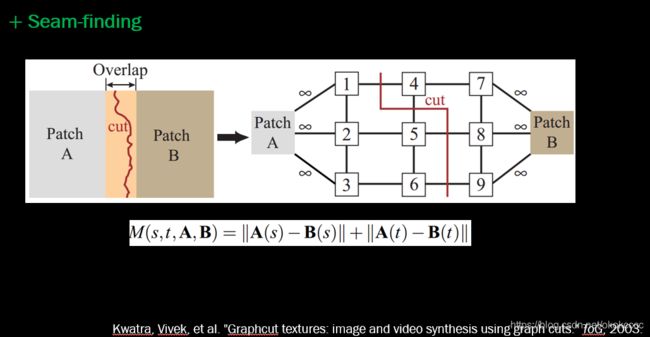
1.3.4 寻找最佳拼接缝
- 很多情况下,使用一个全局单应变换并不能准确对齐图像,需要一些后处理来削弱拼接的痕迹,比如寻找最佳拼接缝【如下图所示】。

- 如何找?
使用最大流最小割算法寻找拼接缝:【找最小割与找最大流在本质上是等价的】
1.4 图像拼接
1.4.1 整体流程
- 根据给定图像/集,实现特征匹配;
- 通过匹配特征计算图像之间的变换结构;
- 利用图像变换结构,实现图像映射;
- 针对叠加后的图像,采用APAP之类的算法,对其特征点;
- 通过图割方法,自动选取拼接缝;
- 根据multu-blending策略实现融合。
1.4.2 multi-blending策略
- multi-band bleing策略采用Laplacian(拉普拉斯)金字塔,通过对相邻两层的高斯金字塔进行差分,将原图分解成不同尺度的子图,对每一个之图进行加权平均,得到每一层的融合结果,最后进行金字塔的反向重建,得到最终融合效果过程,融合之后可以得到较好的拼接效果。

- 如下图所示:

二、全景拼接
2.1 RANSAC
- RANSAC 是“RANdom SAmple Consensus”(随机一致性采样)的缩写。该方法是用来找到正确模型来拟合带有噪声数据的迭代方法。给定一个模型,例如点集之间的单应性矩阵,RANSAC 基本的思想是,数据中包含正确的点和噪声点,合理的模型应该能够在描述正确数据点的同时摒弃噪声点。
- RANSAC的基本假设:
①数据由“局内点”组成,例如:数据的分布可以用一些模型参数来解释;
②“局外点”是不能适应该模型的数据;
③除此之外的数据属于噪声。 - RANSAC算法基本思想:(如上面直线拟合)
①随机选取两个点;
②根据随机选取的两个点构造方程y=ax+b;
③将所有的数据点套到这个模型中计算误差;
④给定阈值,计算inliers数量;
⑤不断重复上述过程,直到达到一次迭代次数后,选择inliers数量最多的直线方程,作为问题的解。 - RANSAC求解单应性矩阵
①随机选择四对匹配特征(选择4对特征点因为单应性矩阵有8个自由度,至少需要8个线性方程求解,对应到点位置信息上,一组点对可以列出两个方程,则至少包含4组匹配点对)
②根据直接线性变换解法DLT计算单应性矩阵H(唯一解)
③对所匹配点,计算映射误差
④根据误差阈值,确定inliers
⑤针对最大的inliers集合,重新计算单应性矩阵H - RANSAC 的标准例子:用一条直线拟合带有噪声数据的点集。简单的最小二乘在该例子中可能会失效,但是 RANSAC 能够挑选出正确的点,然后获取能够正确拟合的直线。
使用RANSAC算法用一条直线来拟合包含噪声点数据点集如下(源自http://www.scopy.org/Cookbook/RANSAC)
【代码】
import numpy
import scipy # use numpy if scipy unavailable
import scipy.linalg # use numpy if scipy unavailable

## Copyright (c) 2004-2007, Andrew D. Straw. All rights reserved.

## Redistribution and use in source and binary forms, with or without
## modification, are permitted provided that the following conditions are
## met:

##     * Redistributions of source code must retain the above copyright
##       notice, this list of conditions and the following disclaimer.

##     * Redistributions in binary form must reproduce the above
##       copyright notice, this list of conditions and the following
##       disclaimer in the documentation and/or other materials provided
##       with the distribution.

##     * Neither the name of the Andrew D. Straw nor the names of its
##       contributors may be used to endorse or promote products derived
##       from this software without specific prior written permission.

## THIS SOFTWARE IS PROVIDED BY THE COPYRIGHT HOLDERS AND CONTRIBUTORS
## "AS IS" AND ANY EXPRESS OR IMPLIED WARRANTIES, INCLUDING, BUT NOT
## LIMITED TO, THE IMPLIED WARRANTIES OF MERCHANTABILITY AND FITNESS FOR
## A PARTICULAR PURPOSE ARE DISCLAIMED. IN NO EVENT SHALL THE COPYRIGHT
## OWNER OR CONTRIBUTORS BE LIABLE FOR ANY DIRECT, INDIRECT, INCIDENTAL,
## SPECIAL, EXEMPLARY, OR CONSEQUENTIAL DAMAGES (INCLUDING, BUT NOT
## LIMITED TO, PROCUREMENT OF SUBSTITUTE GOODS OR SERVICES; LOSS OF USE,
## DATA, OR PROFITS; OR BUSINESS INTERRUPTION) HOWEVER CAUSED AND ON ANY
## THEORY OF LIABILITY, WHETHER IN CONTRACT, STRICT LIABILITY, OR TORT
## (INCLUDING NEGLIGENCE OR OTHERWISE) ARISING IN ANY WAY OUT OF THE USE
## OF THIS SOFTWARE, EVEN IF ADVISED OF THE POSSIBILITY OF SUCH DAMAGE.

def ransac(data,model,n,k,t,d,debug=False,return_all=False):
    """fit model parameters to data using the RANSAC algorithm

This implementation written from pseudocode found at
http://en.wikipedia.org/w/index.php?title=RANSAC&oldid=116358182

{
     {
     {
Given:
    data - a set of observed data points
    model - a model that can be fitted to data points
    n - the minimum number of data values required to fit the model
    k - the maximum number of iterations allowed in the algorithm
    t - a threshold value for determining when a data point fits a model
    d - the number of close data values required to assert that a model fits well to data
Return:
    bestfit - model parameters which best fit the data (or nil if no good model is found)
iterations = 0
bestfit = nil
besterr = something really large
while iterations < k {
    maybeinliers = n randomly selected values from data
    maybemodel = model parameters fitted to maybeinliers
    alsoinliers = empty set
    for every point in data not in maybeinliers {
        if point fits maybemodel with an error smaller than t
             add point to alsoinliers
    }
    if the number of elements in alsoinliers is > d {
        % this implies that we may have found a good model
        % now test how good it is
        bettermodel = model parameters fitted to all points in maybeinliers and alsoinliers
        thiserr = a measure of how well model fits these points
        if thiserr < besterr {
            bestfit = bettermodel
            besterr = thiserr
        }
    }
    increment iterations
}
return bestfit
}}}
"""
    iterations = 0
    bestfit = None
    besterr = numpy.inf
    best_inlier_idxs = None
    while iterations < k:
        maybe_idxs, test_idxs = random_partition(n,data.shape[0])
        maybeinliers = data[maybe_idxs,:]
        test_points = data[test_idxs]
        maybemodel = model.fit(maybeinliers)
        test_err = model.get_error( test_points, maybemodel)
        also_idxs = test_idxs[test_err < t] # select indices of rows with accepted points
        alsoinliers = data[also_idxs,:]
        if debug:
            print 'test_err.min()',test_err.min()
            print 'test_err.max()',test_err.max()
            print 'numpy.mean(test_err)',numpy.mean(test_err)
            print 'iteration %d:len(alsoinliers) = %d'%(
                iterations,len(alsoinliers))
        if len(alsoinliers) > d:
            betterdata = numpy.concatenate( (maybeinliers, alsoinliers) )
            bettermodel = model.fit(betterdata)
            better_errs = model.get_error( betterdata, bettermodel)
            thiserr = numpy.mean( better_errs )
            if thiserr < besterr:
                bestfit = bettermodel
                besterr = thiserr
                best_inlier_idxs = numpy.concatenate( (maybe_idxs, also_idxs) )
        iterations+=1
    if bestfit is None:
        raise ValueError("did not meet fit acceptance criteria")
    if return_all:
        return bestfit, {
     'inliers':best_inlier_idxs}
    else:
        return bestfit

def random_partition(n,n_data):
    """return n random rows of data (and also the other len(data)-n rows)"""
    all_idxs = numpy.arange( n_data )
    numpy.random.shuffle(all_idxs)
    idxs1 = all_idxs[:n]
    idxs2 = all_idxs[n:]
    return idxs1, idxs2

class LinearLeastSquaresModel:
    """linear system solved using linear least squares

    This class serves as an example that fulfills the model interface
    needed by the ransac() function.

    """
    def __init__(self,input_columns,output_columns,debug=False):
        self.input_columns = input_columns
        self.output_columns = output_columns
        self.debug = debug
    def fit(self, data):
        A = numpy.vstack([data[:,i] for i in self.input_columns]).T
        B = numpy.vstack([data[:,i] for i in self.output_columns]).T
        x,resids,rank,s = scipy.linalg.lstsq(A,B)
        return x
    def get_error( self, data, model):
        A = numpy.vstack([data[:,i] for i in self.input_columns]).T
        B = numpy.vstack([data[:,i] for i in self.output_columns]).T
        B_fit = scipy.dot(A,model)
        err_per_point = numpy.sum((B-B_fit)**2,axis=1) # sum squared error per row
        return err_per_point

def test():
    # generate perfect input data

    n_samples = 500
    n_inputs = 1
    n_outputs = 1
    A_exact = 20*numpy.random.random((n_samples,n_inputs) )
    perfect_fit = 60*numpy.random.normal(size=(n_inputs,n_outputs) ) # the model
    B_exact = scipy.dot(A_exact,perfect_fit)
    assert B_exact.shape == (n_samples,n_outputs)

    # add a little gaussian noise (linear least squares alone should handle this well)
    A_noisy = A_exact + numpy.random.normal(size=A_exact.shape )
    B_noisy = B_exact + numpy.random.normal(size=B_exact.shape )

    if 1:
        # add some outliers
        n_outliers = 100
        all_idxs = numpy.arange( A_noisy.shape[0] )
        numpy.random.shuffle(all_idxs)
        outlier_idxs = all_idxs[:n_outliers]
        non_outlier_idxs = all_idxs[n_outliers:]
        A_noisy[outlier_idxs] =  20*numpy.random.random((n_outliers,n_inputs) )
        B_noisy[outlier_idxs] = 50*numpy.random.normal(size=(n_outliers,n_outputs) )

    # setup model

    all_data = numpy.hstack( (A_noisy,B_noisy) )
    input_columns = range(n_inputs) # the first columns of the array
    output_columns = [n_inputs+i for i in range(n_outputs)] # the last columns of the array
    debug = False
    model = LinearLeastSquaresModel(input_columns,output_columns,debug=debug)

    linear_fit,resids,rank,s = scipy.linalg.lstsq(all_data[:,input_columns],
                                                  all_data[:,output_columns])

    # run RANSAC algorithm
    ransac_fit, ransac_data = ransac(all_data,model,
                                     50, 1000, 7e3, 300, # misc. parameters
                                     debug=debug,return_all=True)
    if 1:
        import pylab

        sort_idxs = numpy.argsort(A_exact[:,0])
        A_col0_sorted = A_exact[sort_idxs] # maintain as rank-2 array

        if 1:
            pylab.plot( A_noisy[:,0], B_noisy[:,0], 'k.', label='data' )
            pylab.plot( A_noisy[ransac_data['inliers'],0], B_noisy[ransac_data['inliers'],0], 'bx', label='RANSAC data' )
        else:
            pylab.plot( A_noisy[non_outlier_idxs,0], B_noisy[non_outlier_idxs,0], 'k.', label='noisy data' )
            pylab.plot( A_noisy[outlier_idxs,0], B_noisy[outlier_idxs,0], 'r.', label='outlier data' )
        pylab.plot( A_col0_sorted[:,0],
                    numpy.dot(A_col0_sorted,ransac_fit)[:,0],
                    label='RANSAC fit' )
        pylab.plot( A_col0_sorted[:,0],
                    numpy.dot(A_col0_sorted,perfect_fit)[:,0],
                    label='exact system' )
        pylab.plot( A_col0_sorted[:,0],
                    numpy.dot(A_col0_sorted,linear_fit)[:,0],
                    label='linear fit' )
        pylab.legend()
        pylab.show()

if __name__=='__main__':
    test()
【结果】

【分析】
之所以RANSAC能在有大量噪音情况仍然准确,主要原因是随机取样时只取一部分可以避免估算结果被离群数据影响。
- RANSAC算法的输入为:
- 观测数据 (包括内群与外群的数据)
- 符合部分观测数据的模型 (与内群相符的模型)
- 最少符合模型的内群数量 判断数据是否符合模型的阈值(数据与模型之间的误差容忍度)
- 迭代运算次数 (抽取多少次随机内群)
- RANSAC算法的输出为:
- 最符合数据的模型参数 (如果内群数量小于输入第三条则判断为数据不存在此模型)
- 内群集 (符合模型的数据)
- 优点:
能在包含大量外群的数据中准确地找到模型参数,并且参数不受到外群影响。 - 缺点:
计算参数时迭代次数没有上限,得出来的参数结果有可能并不是最优的,甚至可能不符合真实内群。所以设定 RANSAC参数的时候要根据应用考虑“准确度与效率”哪一个更重要,以此决定做多少次迭代运算。设定与模型的最大误差阈值也是要自己调,因应用而异。还有一点就是RANSAC只能估算一个模型。
2.2 稳健的单应性矩阵估计
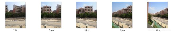
- 在任何模型中都可以使用 RANSAC 模块。在使用 RANSAC 模块时,我们只需要在相应 Python 类中实现fit()和get_error()方法,剩下就是正确地使用ransac.py,我们这里使用可能的对应点集来自动找到用于全景图像的单应性矩阵。下面是使用SIFT特征自动找到匹配对应:
【 代码】
featname = ['C:/Users/ltt/Documents/Subjects/大三下/计算机视觉(蔡国榕)/onepic/match-pic1/' + str(i + 1) + '.sift' for i in range(5)]
imname = ['C:/Users/ltt/Documents/Subjects/大三下/计算机视觉(蔡国榕)/onepic/match-pic1/' + str(i + 1) + '.jpg' for i in range(5)]
# extract features and m
# match
l = {
     }
d = {
     }
for i in range(5):
    sift.process_image(imname[i], featname[i])
    l[i], d[i] = sift.read_features_from_file(featname[i])

matches = {
     }
for i in range(4):
    matches[i] = sift.match(d[i + 1], d[i])

# visualize the matches (Figure 3-11 in the book)
for i in range(4):
    im1 = array(Image.open(imname[i]))
    im2 = array(Image.open(imname[i + 1]))
    figure()
    sift.plot_matches(im2, im1, l[i + 1], l[i], matches[i], show_below=True)
【结果】


2.3 拼接图像
- 估计出图像间的单应性矩阵(使用RANSAC算法),现在我们需要将所有的图像扭曲到一个公共平面上。由于我们所有的图像是由照相机水平旋转拍摄的,因此我们可以使用一个较简单的步骤:将中心图像左边或者右边的区域填充0,以便为扭曲的图像腾出空间。
2.3.1 具体实现
【代码】
from pylab import *
from numpy import *
from PIL import Image

# If you have PCV installed, these imports should work
from PCV.geometry import homography, warp
from PCV.localdescriptors import sift

"""
This is the panorama example from section 3.3.
"""

# set paths to data folder

featname = ['C:/Users/ltt/Documents/Subjects/大三下/计算机视觉(蔡国榕)/onepic/match-pic1/' + str(i + 1) + '.sift' for i in range(5)]
imname = ['C:/Users/ltt/Documents/Subjects/大三下/计算机视觉(蔡国榕)/onepic/match-pic1/' + str(i + 1) + '.jpg' for i in range(5)]
# extract features and m
# match
l = {
     }
d = {
     }
for i in range(5):
    sift.process_image(imname[i], featname[i])
    l[i], d[i] = sift.read_features_from_file(featname[i])

matches = {
     }
for i in range(4):
    matches[i] = sift.match(d[i + 1], d[i])

# visualize the matches (Figure 3-11 in the book)
for i in range(4):
    im1 = array(Image.open(imname[i]))
    im2 = array(Image.open(imname[i + 1]))
    figure()
    sift.plot_matches(im2, im1, l[i + 1], l[i], matches[i], show_below=True)


# function to convert the matches to hom. points
# 将匹配转换成齐次坐标点的函数
def convert_points(j):
    ndx = matches[j].nonzero()[0]
    fp = homography.make_homog(l[j + 1][ndx, :2].T)
    ndx2 = [int(matches[j][i]) for i in ndx]
    tp = homography.make_homog(l[j][ndx2, :2].T)

    # switch x and y - TODO this should move elsewhere
    fp = vstack([fp[1], fp[0], fp[2]])
    tp = vstack([tp[1], tp[0], tp[2]])
    return fp, tp


# estimate the homographies
# 估计单应性矩阵
model = homography.RansacModel()

fp, tp = convert_points(1)
H_12 = homography.H_from_ransac(fp, tp, model)[0]  # im 1 to 2

fp, tp = convert_points(0)
H_01 = homography.H_from_ransac(fp, tp, model)[0]  # im 0 to 1

tp, fp = convert_points(2)  # NB: reverse order
H_32 = homography.H_from_ransac(fp, tp, model)[0]  # im 3 to 2

tp, fp = convert_points(3)  # NB: reverse order
H_43 = homography.H_from_ransac(fp, tp, model)[0]  # im 4 to 3

# 扭曲图像
delta = 2000  # 用于填充和平移 for padding and translation

im1 = array(Image.open(imname[1]), "uint8")
im2 = array(Image.open(imname[2]), "uint8")
im_12 = warp.panorama(H_12, im1, im2, delta, delta)

im1 = array(Image.open(imname[0]), "f")
im_02 = warp.panorama(dot(H_12, H_01), im1, im_12, delta, delta)

im1 = array(Image.open(imname[3]), "f")
im_32 = warp.panorama(H_32, im1, im_02, delta, delta)

im1 = array(Image.open(imname[4]), "f")
im_42 = warp.panorama(dot(H_32, H_43), im1, im_32, delta, 2 * delta)

figure()
imshow(array(im_42, "uint8"))
axis('off')
show()
2.3.2 结果及分析
- 数据集1:
- 结果1:

- 数据集2:

- 结果2:

- 数据集3:

- 结果3:

【分析】 - 以上三组数据集拼接效果都还是可以的,但是由于光影的变化,导致天空的拼接效果不是特别理想,还具有瑕疵;
- 第一组图是宿舍后方,由于照片拍摄的原因,右方距离图片中心较远,导致拼接效果在三组中最差,可以明显的看出拼接的痕迹;
- 第二组图是宿舍楼群,可以看出除了光影处,其余拼接效果较好,无明显痕迹;
- 第三组图是六社区五组团,同样也是光影的问题导致拼接痕迹可以看出。
2.4 小结
结论、问题(及解决方法)
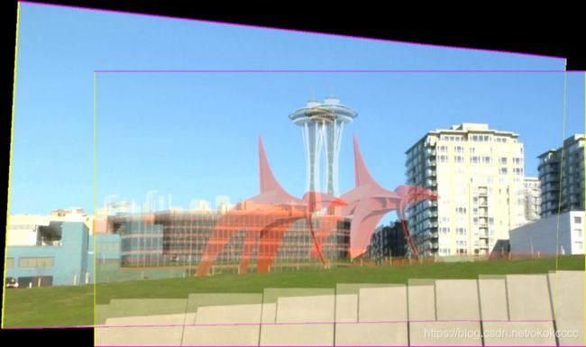
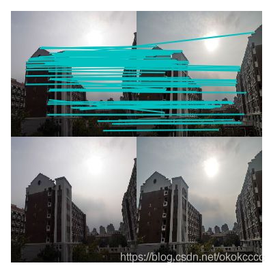
1.在数据集中,图片需按照从右往左开始编号,否则会发生拼接的错乱,如下图所示:

2.图片大小需要调整,否则寻找特征时会发生超出数组索引,且原图较大耗费时间长,最好进行压缩调整;
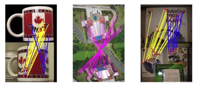
3.选取数据集图片时,要选取特征点明显,较为好匹配的,且要遵循拼接图片规则,否则会遇到这个错误:ValueError: did not meet fit acceptance criteria如下图数据集便是不可取的:

4.正如以上实验所看见的,图像曝光不同,在单个图像的边界上存在边缘效应,导致拼接痕迹较为明显。(商业的创建全景图像软件里有额外的操作来对强度进行归一化,并对平移进行平滑场景转换,以使得结果看上去更好。)