高光谱图像pca降维_高光谱图像的显示
spectral python的主页在:Welcome to Spectral Python (SPy)
Spy中包括从安装,图像显示、高光谱图像处理算法等的全套API的内容。
我们这里只关注一下高光谱图像的显示。
spectral python的命令时基于ipython的,因此,如果以命令行脚本的形式使用spectral python,则需要首先进入ipython的环境。进入方法如下:
ipython --pylab=wx
下面我贴出来一个可以显示高光谱原始图像,原始图像和groud_truth的混合图像,以及显示光谱立方体的脚本。
如下脚本:
In [1]: import matplotlib.pyplot as plt
...: import scipy.io as sio
...: import os
...: import spectral
第[1]句是加载需要用到的软件包
In [2]: data_path = os.path.join(os.getcwd(), 'data')
#第【3】句,加载mat格式保存的高光谱数据Indian_pines_corrected.mat
In [3]: data = sio.loadmat(os.path.join(data_path, 'Indian_pines_corrected.mat'))['indian_pines_corrected']
#加载mat格式保存的对应ground_truth
In [4]: labels = sio.loadmat(os.path.join(data_path, 'Indian_pines_gt.mat'))['indian_pines_gt'] ...:
In [5]: img = data
In [6]: gt = labels
同时显示原高光谱图像中的30,20,10通道和groundtruth,以覆盖的方式显示,透明度为0.5.
In [7]: view = spectral.imshow(img, (30, 20, 10), classes=gt)
In [8]: view.set_display_mode('overlay')
In [9]: view.class_alpha = 0.5

以超立方体的形式显示高光谱图像
In [10]: spectral.view_cube(img,bands=[29, 19, 9])
Out[10]:

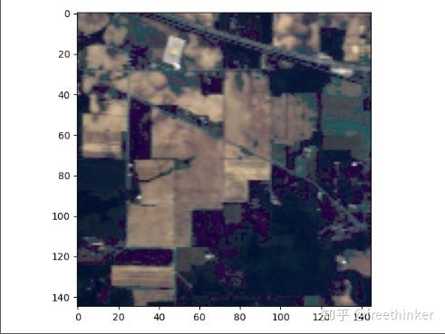
将高光谱图象中的29,19,9波段,分别作为r,g,b分量的值,显示出一幅彩色图。
imshow()有两个参数,一个是data,图像,存储格式需要是np.ndarray或者SpyFile。
另一个参数bonds,是显示的波段,从多个波段中选择3个,作为rgb三个分量的输入进行选择。
If `bands` has 3 values, the bands specified are extracted from`data` to be plotted as the red, green, and blue colors,
In[11]: spectral.imshow(img,(29, 19, 9))
上述显示整理为一个python文件,源码如下:
import matplotlib.pyplot as plt
import http://scipy.io as sio
import os
import spectral
os.environ["CUDA_VISIBLE_DEVICES"] = "3"
## GLOBAL VARIABLES
dataset = 'IP'
test_ratio = 0.7
windowSize = 25
def loadData(name):
data_path = os.path.join(os.getcwd(), 'data')
if name == 'IP':
data = sio.loadmat(os.path.join(data_path, 'Indian_pines_corrected.mat'))['indian_pines_corrected']
labels = sio.loadmat(os.path.join(data_path, 'Indian_pines_gt.mat'))['indian_pines_gt']
elif name == 'SA':
data = sio.loadmat(os.path.join(data_path, 'Salinas_corrected.mat'))['salinas_corrected']
labels = sio.loadmat(os.path.join(data_path, 'Salinas_gt.mat'))['salinas_gt']
elif name == 'PU':
data = sio.loadmat(os.path.join(data_path, 'PaviaU.mat'))['paviaU']
labels = sio.loadmat(os.path.join(data_path, 'PaviaU_gt.mat'))['paviaU_gt']
return data, labels
X, y = loadData(dataset)
print(X.shape, y.shape)
view = spectral.imshow(X, (29, 19, 9))
#view = spectral.imshow(X, (1, 2, 3))
print(view)
plt.show()
#show grandtruth
gt_view = spectral.imshow(classes=y)
plt.show()
#show both the data and the class value
img = X
gt = y
view = spectral.imshow(img, (30, 20, 10), classes=gt)
view.set_display_mode('overlay')
view.class_alpha = 0.5
plt.show()
#saving rgb image files
spectral.save_rgb('rgb.jpg', img, [29, 19, 9])
spectral.save_rgb('gt.jpg', gt, colors=spectral.spy_colors)
#spectral.view_cube(img, spectral.bands=[29, 19, 9])
spectral.view_cube(img,bands=[29, 19, 9])
plt.show()
#注意上面python文件在pycharm中运行显示超立方体,我这边没有显示成功。