YOLO 训练可视化：loss、iou、F1、map、precision、recall

保存训练日志

在命令最后加上：>>train.log 或者 | tee train.log
训练过程就会生成一个log文件。

提取log文件

在log文件目录下，新建 extract_log.py 脚本：

# coding=utf-8
# 该文件用来提取训练log，去除不可解析的log后使log文件格式化，生成新的log文件供可视化工具绘图
 
import inspect
import os
import random
import sys
def extract_log(log_file,new_log_file,key_word):
    with open(log_file, 'r',encoding='utf-16LE') as f:
      with open(new_log_file, 'w') as train_log:
  #f = open(log_file)
    #train_log = open(new_log_file, 'w')
        for line in f:
    # 去除多gpu的同步log
          if 'Syncing' in line:
            continue
    # 去除除零错误的log
          if 'nan' in line:
            continue
          if key_word in line:
            train_log.write(line)
    f.close()
    train_log.close()
 
extract_log('train_yolov3.log','train_log_loss.txt','images')
extract_log('train_yolov3.log','train_log_iou.txt','IOU')
extract_log('train_yolov3.log','train_log_map.txt','[email protected]') 
extract_log('train_yolov3.log','train_log_F1.txt','F1-score')

运行之后将会生成：train_log_loss.txt、train_log_iou.txt、train_log_map.txt、train_log_F1.txt 四个文件。

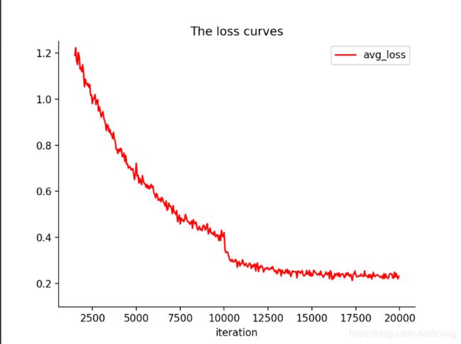
loss曲线

新建visualization_loss.py脚本：根据自己要求修改

import pandas as pd
import numpy as np
import matplotlib.pyplot as plt
#%matplotlib inline
 
lines =20000    #改为自己生成的train_log_loss.txt中的行数
start_ite = 1 #log_loss.txt里面的最小迭代次数
end_ite = 20000 #log_loss.txt里面的最大迭代次数
step = 50 #跳行数，决定画图的稠密程度
igore = 1500 #当开始的loss较大时，你需要忽略前igore次迭代，注意这里是迭代次数
result = pd.read_csv('train_log_loss.txt',skiprows=[x for x in range(lines) if (x<lines*1.0/((end_ite - start_ite)*1.0)*igore or x%step!=9)]\
    , error_bad_lines=False, names=['loss', 'avg', 'rate', 'seconds', 'images'])
result.head()
 
result['loss']=result['loss'].str.split(' ').str.get(1)
result['avg']=result['avg'].str.split(' ').str.get(1)
result['rate']=result['rate'].str.split(' ').str.get(1)
result['seconds']=result['seconds'].str.split(' ').str.get(1)
result['images']=result['images'].str.split(' ').str.get(1)


result['loss']=pd.to_numeric(result['loss'],errors='ignore')
result['avg']=pd.to_numeric(result['avg'],errors='ignore')
result['rate']=pd.to_numeric(result['rate'],errors='ignore')
result['seconds']=pd.to_numeric(result['seconds'],errors='ignore')
result['images']=pd.to_numeric(result['images'],errors='ignore')

x_num = len(result['avg'].values)
tmp = (end_ite-start_ite - igore)/(x_num*1.0)
x = []
for i in range(x_num):
	x.append(i*tmp + start_ite + igore)

fig = plt.figure(1, dpi=160)
ax = fig.add_subplot(1, 1, 1)
ax.plot(x,result['avg'].values,'r', label='avg_loss')
ax.legend(loc='best')
ax.set_ylim([0.1, 1.25])
#ax.set_xlim([0, 200])
ax.set_title('The loss curves')
ax.set_xlabel('iteration')
ax.spines['top'].set_visible(False)     #去掉上边框
ax.spines['right'].set_visible(False)   #去掉右边框
fig.savefig('avg_loss')

运行后将会生成loss曲线

iou曲线

新建visualization_iou.py脚本：

#!/usr/bin/python
#coding=utf-8
 
import pandas as pd
import numpy as np
import matplotlib.pyplot as plt
 
#根据log_iou修改行数
lines = 588539
step = 5000
start_ite = 0
end_ite = 20000
igore = 100
data_path =  'train_log_iou.txt' #log_loss的路径。
result_path = 'Region Avg IOU' #保存结果的路径。
 
names = ['Region Avg IOU', 'Class', 'Obj', 'No Obj', '.5_Recall', '.7_Recall', 'count']
#result = pd.read_csv('log_iou.txt', skiprows=[x for x in range(lines) if (x%10==0 or x%10==9)]\
result = pd.read_csv(data_path, skiprows=[x for x in range(lines) if (x<lines*1.0/((end_ite - start_ite)*1.0)*igore or x%step!=0)]\
, error_bad_lines=False, names=names)
result.head()
 
for name in names:
    result[name] = result[name].str.split(': ').str.get(1)
result.head()
result.tail()
for name in names:
    result[name] = pd.to_numeric(result[name])
result.dtypes
 
 
####--------------
x_num = len(result['Region Avg IOU'].values)
tmp = (end_ite-start_ite - igore)/(x_num*1.0)
x = []
for i in range(x_num):
	x.append(i*tmp + start_ite + igore)
#print(x)
print('total = %d\n' %x_num)
print('start = %d, end = %d\n' %(x[0], x[-1]))
####-------------
 
 
fig = plt.figure()
ax = fig.add_subplot(1,1,1)
ax.plot(x, result['Region Avg IOU'].values, label='Region Avg IOU')
#ax.plot(result['Avg Recall'].values, label='Avg Recall')
plt.grid()
ax.legend(loc='best')
ax.set_title('The Region Avg IOU curves')
ax.set_xlabel('batches')
fig.savefig(result_path)

运行后即可生成IOU曲线

下面的F1、map、precision、recall四条曲线都是在train_log_F1.txt文件内提取相关数据得到的。代码基本相同，只需修改相关字符就行。

F1曲线

#!/usr/bin/python
#coding=utf-8
 
import pandas as pd
import numpy as np
import matplotlib.pyplot as plt

 
#根据log_iou修改行数
lines = 191
step = 1
start_ite = 0
end_ite = 191
igore = 0
data_path =  'train_log_F1.txt' #f1的路径。
result_path = 'F1' #保存结果的路径。
 
names = ['conf_thresh', 'precision', 'recall', 'F1-score']
#result = pd.read_csv('log_iou.txt', skiprows=[x for x in range(lines) if (x%10==0 or x%10==9)]\
result = pd.read_csv(data_path, skiprows=[x for x in range(lines) if (x<lines*1.0/((end_ite - start_ite)*1.0)*igore or x%step!=0)]\
, error_bad_lines=False, names=names)
result.head()
for name in names:
    result[name] = result[name].str.split(' = ').str.get(1)
result.head()
result.tail()
for name in names:
    result[name] = pd.to_numeric(result[name])
result.dtypes
 
 
####--------------
x_num = len(result['F1-score'].values)
tmp = (end_ite-start_ite - igore)/(x_num*1.0)
x = []
for i in range(x_num):
	x.append(i*tmp + start_ite + igore)
#print(x)
print('total = %d\n' %x_num)
print('start = %d, end = %d\n' %(x[0], x[-1]))
####-------------
 
 
fig = plt.figure(1, dpi=160)
ax = fig.add_subplot(1,1,1)
ax.plot(x, result['F1-score'].values, 'r',label='F1-score')
#ax.plot(result['Avg Recall'].values, label='Avg Recall')
#plt.grid()
ax.legend(loc='best')
ax.set_ylim([0.4, 0.85])
ax.set_xlim([-5, 200])
ax.set_title('The F1-score curves')
ax.set_xlabel('batches')
ax.spines['top'].set_visible(False)     #去掉上边框
ax.spines['right'].set_visible(False)   #去掉右边框
fig.savefig(result_path)

map曲线

#!/usr/bin/python
#coding=utf-8
 
import pandas as pd
import numpy as np
import matplotlib.pyplot as plt
 
#根据log_iou修改行数
lines = 191
step = 1
start_ite = 0
end_ite = 191
igore = 0
data_path =  'train_log_map.txt' #f1的路径。
result_path = 'map' #保存结果的路径。
 
names = ['([email protected])', 'or']
#result = pd.read_csv('log_iou.txt', skiprows=[x for x in range(lines) if (x%10==0 or x%10==9)]\
result = pd.read_csv(data_path, skiprows=[x for x in range(lines) if (x<lines*1.0/((end_ite - start_ite)*1.0)*igore or x%step!=0)]\
, error_bad_lines=False, names=names)
result.head()
 
for name in names:
    result[name] = result[name].str.split(' = ').str.get(1)
result.head()
result.tail()
for name in names:
    result[name] = pd.to_numeric(result[name])
result.dtypes
 
 
####--------------
x_num = len(result['([email protected])'].values)
tmp = (end_ite-start_ite - igore)/(x_num*1.0)
x = []
for i in range(x_num):
	x.append(i*tmp + start_ite + igore)
#print(x)
print('total = %d\n' %x_num)
print('start = %d, end = %d\n' %(x[0], x[-1]))
####-------------
 
 
fig = plt.figure()
ax = fig.add_subplot(1,1,1)
ax.plot(x, result['([email protected])'].values, label='mAP')
#ax.plot(result['Avg Recall'].values, label='Avg Recall')
plt.grid()
ax.legend(loc='best')
ax.set_title('The mAP curves')
ax.set_xlabel('epoch')
fig.savefig(result_path)

precision曲线

#!/usr/bin/python
#coding=utf-8
 
import pandas as pd
import numpy as np
import matplotlib.pyplot as plt
 
#根据log_iou修改行数
lines = 191
step = 1
start_ite = 0
end_ite = 191
igore = 0
data_path =  'train_log_F1.txt' #f1的路径。
result_path = 'precision' #保存结果的路径。
 
names = ['conf_thresh', 'precision', 'recall', 'F1-score']
#result = pd.read_csv('log_iou.txt', skiprows=[x for x in range(lines) if (x%10==0 or x%10==9)]\
result = pd.read_csv(data_path, skiprows=[x for x in range(lines) if (x<lines*1.0/((end_ite - start_ite)*1.0)*igore or x%step!=0)]\
, error_bad_lines=False, names=names)
result.head()
 
for name in names:
    result[name] = result[name].str.split(' = ').str.get(1)
result.head()
result.tail()
for name in names:
    result[name] = pd.to_numeric(result[name])
result.dtypes
 
 
####--------------
x_num = len(result['precision'].values)
tmp = (end_ite-start_ite - igore)/(x_num*1.0)
x = []
for i in range(x_num):
	x.append(i*tmp + start_ite + igore)
#print(x)
print('total = %d\n' %x_num)
print('start = %d, end = %d\n' %(x[0], x[-1]))
####-------------
 
 
fig = plt.figure()
ax = fig.add_subplot(1,1,1)
ax.plot(x, result['precision'].values, label='precision')
#ax.plot(result['Avg Recall'].values, label='Avg Recall')
plt.grid()
ax.legend(loc='best')
ax.set_title('The precision curves')
ax.set_xlabel('batches')
fig.savefig(result_path)

recall曲线

#!/usr/bin/python
#coding=utf-8
 
import pandas as pd
import numpy as np
import matplotlib.pyplot as plt
 
#根据log_iou修改行数
lines = 191
step = 1
start_ite = 0
end_ite = 191
igore = 0
data_path =  'train_log_F1.txt' #f1的路径。
result_path = 'recall' #保存结果的路径。
 
names = ['conf_thresh', 'precision', 'recall', 'F1-score']
#result = pd.read_csv('log_iou.txt', skiprows=[x for x in range(lines) if (x%10==0 or x%10==9)]\
result = pd.read_csv(data_path, skiprows=[x for x in range(lines) if (x<lines*1.0/((end_ite - start_ite)*1.0)*igore or x%step!=0)]\
, error_bad_lines=False, names=names)
result.head()
 
for name in names:
    result[name] = result[name].str.split(' = ').str.get(1)
result.head()
result.tail()
for name in names:
    result[name] = pd.to_numeric(result[name])
result.dtypes
 
 
####--------------
x_num = len(result['recall'].values)
tmp = (end_ite-start_ite - igore)/(x_num*1.0)
x = []
for i in range(x_num):
	x.append(i*tmp + start_ite + igore)
#print(x)
print('total = %d\n' %x_num)
print('start = %d, end = %d\n' %(x[0], x[-1]))
####-------------
 
 
fig = plt.figure()
ax = fig.add_subplot(1,1,1)
ax.plot(x, result['recall'].values, label='recall')
#ax.plot(result['Avg Recall'].values, label='Avg Recall')
plt.grid()
ax.legend(loc='best')
ax.set_title('The recall curves')
ax.set_xlabel('batches')
fig.savefig(result_path)

运行以上代码即可得到相应曲线。

参考链接：
YOLO-V3可视化训练过程中的参数，绘制loss、IOU、avg Recall等的曲线图
win10 + YOLOv3 在darknet下可视化训练过程的参数