吴恩达机器学习课后作业——线性回归（Python实现）

1.写在前面

吴恩达机器学习的课后作业及数据可以在coursera平台上进行下载，只要注册一下就可以添加课程了。所以这里就不写题目和数据了，有需要的小伙伴自行去下载就可以了。
作业及数据下载网址：吴恩达机器学习课程

2.单变量线性回归

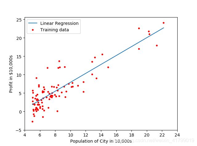
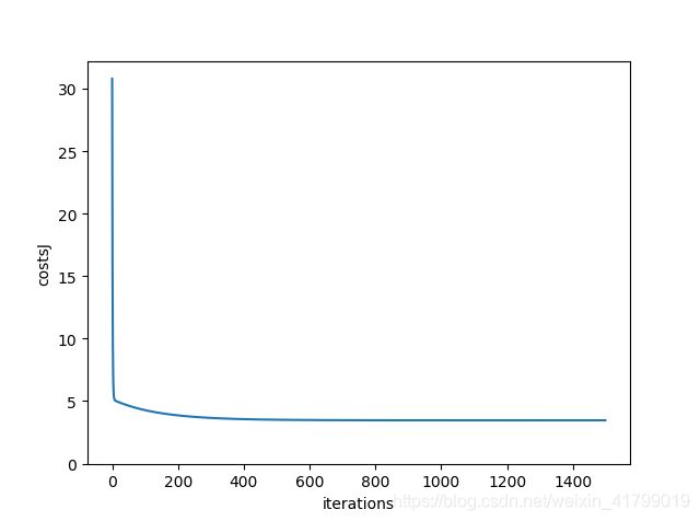
单变量的线性回归的作业主要包含两个任务：进行拟合函数的绘制以及展示梯度下降的过程。下面附上代码，有详细的注释，这里就不一一解释了。

import pandas as pd
import numpy as np
import matplotlib
import matplotlib.pyplot as plt

#用于导入数据的函数
def inputData():
    data=pd.read_csv('MachineLearning\\machine-learning-ex1\\machine-learning-ex1\\ex1\\ex1data1.txt')
    data.insert(0,'ones',[1 for i in range(0,data.shape[0])])   #在dataframe在第一列中加入全为1的列
    #以下是将dataframe中的数据转换为矩阵
    X=data.iloc[:,0:2]      #取出第1-2列的数据作为自变量
    X=X.values
    y=data.iloc[:,2]        #取出第3列的数据作为因变量
    y=y.values
    y=y.reshape(y.shape[0],1)   #注意这里，一行的数据最好使用reshape方法重构成向量，方便之后处理
    return X,y

#用于计算代价函数
def computingTheCost(m,X,y):
    costJ=(pow((X@theta-y),2)).sum()/(2*m)      #根据吴恩达老师视频中的公式进行推导所得
    return costJ

#用于进行梯度下降的函数
def gradientDescent(m,X,y,costs):
    for k in range(0,iterations):           #进行迭代
        #以下完全根据吴恩达老师视频中进行编写代码
        #使用@表示矩阵相乘，使用*表示两个同形矩阵对应数值相乘   
        temp0=theta[0]-alpha*(X@theta-y).sum()/m     
        temp1=theta[1]-alpha*((X@theta-y)*X[:,1].reshape(X.shape[0],1)).sum()/m     #注意这里一定要将X[:,1]reshape成向量
        costs[k]=computingTheCost(m,X,y)        #调用计算代价的函数，记录当前的代价数值
        theta[0]=temp0                  #进行同步更新θ0和θ1
        theta[1]=temp1
    return theta,costs

#用于展示拟合函数
def showPrediction(X,y,theta):
    c1=theta[0]     #从theta中获得第一个参数θ0
    c2=theta[1]     #从theta中获得第二个参数θ1
    xx=np.linspace(np.min(X[:,1]),np.max(X[:,1]),100)       #使用linspace函数生成间隔均匀的数字
    yy=c1+c2*xx     #建立预测的表达式
    #下面就是对于散点图以及拟合函数的绘制
    plt.plot(xx,yy,label='Linear Regression')                   #绘制拟合函数
    plt.scatter(X[:,1],y,c='red',marker='.',label='Training data')  #绘制散点图
    plt.xlabel('Population of City in 10,000s')
    plt.ylabel('Profit in $10,000s')
    x_ticks=np.arange(4,26,2)
    y_ticks=np.arange(-5,30,5)
    plt.xticks(x_ticks)
    plt.yticks(y_ticks)
    plt.legend(loc='best')
    plt.show()

#展示梯度下降的情况
def showGradientDescent(costs,iterations):
    #通过之前计算的代价函数，使用可视化的形式展现随着迭代的进行，代价函数下降的过程
    plt.plot(np.arange(0,iterations,1),costs)
    plt.xticks(np.arange(0,1600,200))
    plt.yticks(np.arange(0,35,5))
    plt.xlabel('iterations')
    plt.ylabel('costsJ')
    plt.show()



X,y=inputData()         #导入数据
theta=np.zeros((2,1))   #使用0初始化θ数组
iterations=1500         #定义迭代的次数
alpha=0.02              #定义学习率α
costs=np.array([0.1 for i in range(0,iterations)])      #创建代价函数数组
theta,costs=gradientDescent(X.shape[0],X,y,costs)       #进行梯度下降，返回最优θ和代价函数值

#showPrediction(X,y,theta)             #用于展示拟合函数
#showGradientDescent(costs,iterations)     #用于展示梯度下降的过程

结果展示：

3.多变量线性回归

单变量的线性回归的作业主要包含两个任务：对不同的学习率的梯度下降情况进行展示、分别利用正规方程和梯度下降进行预测。下面附上代码，有详细的注释，这里就不一一解释了。

import numpy as np
import matplotlib.pyplot as plt
import pandas as pd

#用于导入数据的函数
def inputData():
    #注意这里最好指明导入数据的类型，因为后面会涉及到正规化，int和float不太一样
    data=pd.read_csv('MachineLearning\\machine-learning-ex1\\machine-learning-ex1\\ex1\\ex1data2.txt'
                ,dtype={
     0:float,1:float,2:float}) 
    ##在dataframe在第一列中加入全为1的列  
    data.columns=['size of house','num of room','price of room']
    data.insert(0,'one',[1 for i in range(0,data.shape[0])])
    #以下是将dataframe中的数据转换为矩阵
    X=data.iloc[:,0:3]      #取出第1-3列的数据作为自变量
    X=X.values
    y=data.iloc[:,3]        #取出第4列的数据作为因变量
    y=y.values
    y=y.reshape(46,1)       #注意这里，一行的数据最好使用reshape方法重构成向量，方便之后处理
    return X,y

#用于进行特征缩放的函数（均值归一化）
def featureNormalize(data,b):
    for i in range(0,b):
        dataMean = np.mean(data[:,i])       #获取第i列的平均值
        dataStd  = np.std(data[:,i])        #获取第i列的标准差
        for j in range(0,data.shape[0]):    #遍历第i列中每一个数值
            data[j,i] = (data[j,i]-dataMean)/dataStd        #利用吴恩达老师的公式进行归一化
    return data

#用于计算代价函数
def costs(m,theta,X,y):
    costsJ= pow(X@theta-y,2).sum()/(2*m)    #根据吴恩达老师视频中的公式进行推导所得
    return costsJ

#用于进行梯度下降的函数
def gradientDescent(m,theta,alpha,iterations,X,y,costsC):
    for i in range(0,iterations):       #进行迭代
        #以下完全根据吴恩达老师视频中进行编写代码
        #使用@表示矩阵相乘，使用*表示两个同形矩阵对应数值相乘   
        temp0=theta[0]-alpha*((X@theta-y)*X[:,0].reshape(X.shape[0],1)).sum()/m  #注意这里一定要将X[:,1]reshape成向量
        temp1=theta[1]-alpha*((X@theta-y)*X[:,1].reshape(X.shape[0],1)).sum()/m
        temp2=theta[2]-alpha*((X@theta-y)*X[:,2].reshape(X.shape[0],1)).sum()/m
        costsC[0,i]=costs(m,theta,X,y)      #调用计算代价的函数，记录当前的代价数值
        theta[0]=temp0          #进行同步更新θ0和θ1和θ2
        theta[1]=temp1
        theta[2]=temp2
    return costsC,theta

#用正规方程进行计算的函数
def normalEquation(X,y):
    #利用numpy的linalg的线代函数库根据公式进行计算
    return np.linalg.inv(X.T@X)@X.T@y   

#利用正规方程的方法进行预测的函数
def predictThroughNormalEquation(X,y,size,num):
    finaltheta=normalEquation(X,y)      #调用正规方程的函数
    predictValue=finaltheta[0][0]+finaltheta[1][0]*size+finaltheta[2][0]*num  #构造表达式计算结果
    print('predictThroughNormalEquation=',predictValue)

#展示不同学习率α的梯度下降情况
def showGradientDescent(X,y):
    answer1 = featureNormalize(X[:,1:3],2)      #调用归一化的函数
    X[:,1]=answer1[:,0]         #将结果写入X中
    X[:,2]=answer1[:,1]
    costsC=np.zeros((4,iterations))     #建立4个代价函数costs数组
    for i in range(0,4):                #分别遍历四种学习率α
        temp=np.zeros((1,iterations))   #初始化一个临时的代价数组
        theta=np.zeros((3,1))           #初始化一个θ数组
        temp,theta = gradientDescent(X.shape[0],theta,alpha[i],iterations,X,y,temp)     #调用梯度下降函数
        costsC[i]=temp                  #将temp返回给代价函数数组

    #下面就是用于展示四种学习率α的下降情况
    x=np.arange(0,iterations)           
    plt.plot(x,costsC[0],c='r',label='alpha=0.3')
    plt.plot(x,costsC[1],c='b',label='alpha=0.1')
    plt.plot(x,costsC[2],c='y',label='alpha=0.03')
    plt.plot(x,costsC[3],c='g',label='alpha=0.01')
    plt.legend(loc="best")
    plt.show()

#利用梯度下降的方法进行预测的函数
def predictThroughGradientDescent(X,y,size,num):
    #特别注意：在进行预测的时候，同样需要对预测的size和num进行归一化
    sizeMean = np.mean(X[:,1])      #计算房子大小的均值
    sizeStd = np.std(X[:,1])        #计算房子大小的标准差
    numMean  = np.mean(X[:,2])      #计算房间数量的均值
    numStd  = np.std(X[:,2])        #计算房间数量的标准差
    normalSize=(size-sizeMean)/sizeStd  #房子大小归一化
    normalnum=(num-numMean)/numStd      #房间数量归一化

    answer1 = featureNormalize(X[:,1:3],2)  #对房子大小和房间数量进行归一化
    X[:,1]=answer1[:,0]
    X[:,2]=answer1[:,1]
    alpha=0.3                       #因为从比较上看，学习率0.3是效果最好的，所以这里选用0.3
    costsC=np.zeros((1,iterations))     #初始化代价函数数组
    theta=np.zeros((3,1))           #初始化θ数组
    costsC,theta=gradientDescent(X.shape[0],theta,alpha,iterations,X,y,costsC)      #进行梯度下降
    predictValue=theta[0][0]+theta[1][0]*normalSize+theta[2][0]*normalnum   #构造预测表达式
    print('predictThroughGradientDescent=',predictValue)        #打印预测值

alpha=[0.3,0.1,0.03,0.01]       #学习率α数组
iterations=15                 #迭代次数
X,y=inputData()                 #输入数据

# showGradientDescent(X,y)         #展示不同学习率α的梯度下降情况
predictThroughNormalEquation(X,y,2400,3)      #使用正规方程进行预测
predictThroughGradientDescent(X,y,2400,3)     #使用梯度下降进行预测

结果展示：