定位步骤
卡尔曼滤波器
回顾一下卡尔曼用语定位的步骤:
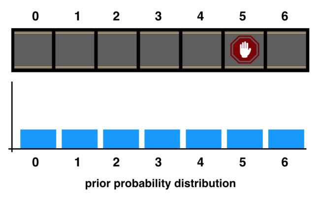
- 初步预测
下面是一个例子,我们知道我们的车在这条单车道上,但我们不知道它的确切位置。
-
测量更新
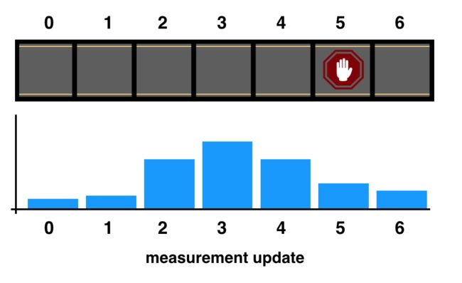
感知周围的世界称之为测量更新。收集有关汽车周围环境的更多信息并改进我们的预测。
比如:测量的停车标志前两个网格单元,测量并不完美,但我们对汽车的位置有了更好的了解。
-
预测(时间更新)
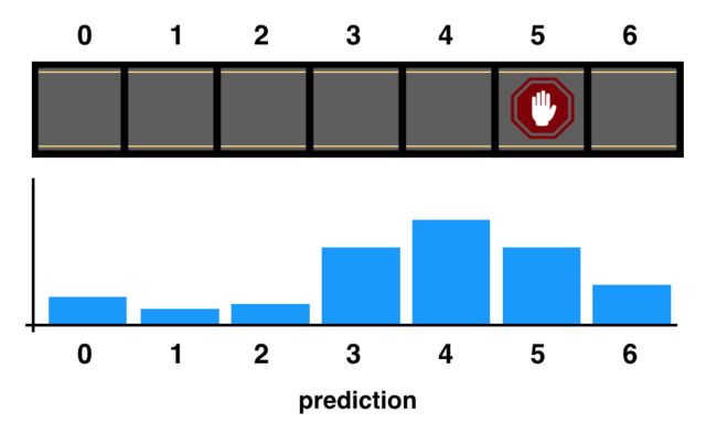
下一步是移动,也称之为时间更新或预测步骤;我们根据对速度和当前位置的了解,预测汽车的移动位置。
比如:将概率分布向右移动一个单元格
-
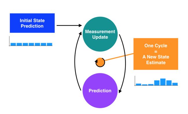
循环重复
已经形成了对汽车位置的新估计,卡尔曼滤波器简单的重复感应和移动(测量和预测),以便在汽车移动时对汽车进行定位!
卡尔曼滤波器可以结合不准确的传感器测量和稍微不准确的运动预测,以获得比仅来自传感器读数或仅有关运动的任何更好估计位置。
状态
当定位一辆汽车时,汽车位置和运动通常被称为汽车状态。
汽车的状态包括:汽车当前位置X以及速度
X= 0
velocity = 50
initial_state = [x, velocity]
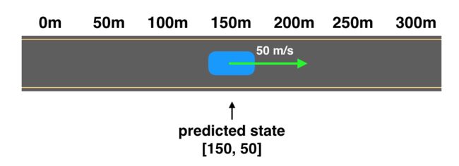
假如汽车行驶在一条单行道上:
汽车当前位置在这条路起点,以每秒50米的速度前进,因此三秒后,它将达到150米标记处
运动模型
以上是一个合理的预测,有以下假设:
- 汽车有一个初始状态
- 假设汽车以一个恒定速度前进
distance = velocity * time该等式也称之为运动模型
一个更复杂的模型:
汽车依旧从零点出发,此时的速度为50米每秒,但它以-20m/s2的加速度速度递减
为了解决这个问题:在状态中包含一个新值:加速度
- distance = velocitydt + 0.5acceleration*dt2
- velocity = acceleration * dt
状态包括此模型中的加速度,如下所示:[x, velocity, acc]。
# Constant acceleration, changing velocity

# initial variables
x = 0
velocity = 50
acc = -20

initial_state = [x, velocity, acc]

# predicted state after three seconds have elapsed
# this state has a new value for x, and a new value for velocity (but the acceleration stays the same)
dt = 3

new_x = x + velocity*dt + 0.5*acc*dt**2
new_vel = velocity + acc*dt

predicted_state = [new_x, new_vel, acc]  # predicted_state = [60, -10, -20]
#---- predict state function --#
def predict_state(state, dt):
    # Assumes a valid state had been passed in
    # Assumes a constant velocity model
    x = state[0]
    new_x = x+state[1]*dt

    # Create and return the new, predicted state
    predicted_state = [new_x, state[1]]
    return predicted_state
from functions import predict_state

# predict_state takes in a state and a change in time, dt
# So, a call might look like: new_state = predict_state(old_state, 2)

# The car starts at position = 0, going 60 m/s
# The initial state:
initial_state = [10, 60]

# After 2 seconds:
state_est1 = predict_state(initial_state, 2)

# 3 more seconds after the first estimated state
state_est2 = predict_state(state_est1, 3)

## TODO: Use the predict_state function
## and the above variables to calculate the following states
## (And change their value from 0 to the correct state)

## Then, click Test Run to see your results!

## 1 more second after the second state estimate
state_est3 = predict_state(state_est2, 1)

## 4 more seconds after the third estimated state
state_est4 =  predict_state(state_est3, 4)
汽车对象
创建汽车对象
状态由位置定义:[y,x];速度具有垂直分量和水平分量:[vy,vx]
import matplotlib.pyplot as plt

""" The Car class defines a car's movement and keeps track of its state.

    The class includes init, move, and display functions.
    This class assumes a constant velocity motion model and the state
    of the car includes the car's position, and it's velocity.

    Attributes:
        state: A list of the car's current position [y, x] and velocity [vy, vx]
        world: The world that the car is moving within (a 2D list)
"""

class Car(object):


    # Car constructor
    # Called when you write car.Car(_, _, _)
    def __init__(self, position, velocity, world):
        """Initializes Car with some position, velocity, and a world to traverse."""

        # Initialize the state
        # Position is a list [y, x] and so is velocity [vy, vx]
        self.state = [position, velocity]
        self.world = world # world is a 2D list of values that range from 0-1

        # Set the default color
        self.color = 'r'

        # Initalize the path
        self.path = []
        self.path.append(position)


    # Move function
    def move(self, dt=1):
        """ The move function moves the car in the direction of the velocity and
            updates the state.
            It assumes a circular world and a default dt = 1 (though dt can be any
            non-negative integer).
            """

        height = len(self.world)
        width = len(self.world[0])

        position = self.state[0]
        velocity = self.state[1]

        # Predict the new position [y, x] based on velocity [vx, vy] and time, dt
        predicted_position = [
            (position[0] + velocity[0]*dt) % height, # default dt = 1
            (position[1] + velocity[1]*dt) % width
        ]

        # Update the state
        self.state = [predicted_position, velocity]

        # Every time the robot moves, add the new position to the path
        self.path.append(predicted_position)


    # Turn left function
    def turn_left(self):
        """ Turning left "rotates" the velocity values, so vy = -vx, and vx = vy.

            For example, if a car is going right at 1 world cell/sec this means
            vy = 0, vx = 1,
            and if it turns left, then it should be moving upwards on the world grid
            at the same speed!
            And up is vy = -1 and vx = 0
            """

        # Change the velocity
        velocity = self.state[1]

        predicted_velocity = [
            -velocity[1],
            velocity[0]
        ]

        # Update the state velocity
        self.state[1] = predicted_velocity


    ## TODO: Write the turn_right function
    ## Hint: Use turn_left for inspiration!
    def turn_right(self):
        """ Turning left "rotates" the velocity values, so vy = -vx, and vx = vy.

            For example, if a car is going right at 1 world cell/sec this means
            vy = 0, vx = 1,
            and if it turns left, then it should be moving upwards on the world grid
            at the same speed!
            And up is vy = -1 and vx = 0
            """

        # Change the velocity
        velocity = self.state[1]

        predicted_velocity = [
            velocity[1],
            -velocity[0]
        ]

        # Update the state velocity
        self.state[1] = predicted_velocity


    # Helper function for displaying the world + robot position
    # Assumes the world in a 2D numpy array and position is in the form [y, x]
    # path is a list of positions, and it's an optional argument
    def display_world(self):

        # Store the current position of the car
        position = self.state[0]

        # Plot grid of values + initial ticks
        plt.matshow(self.world, cmap='gray')

        # Set minor axes in between the labels
        ax=plt.gca()
        rows = len(self.world)
        cols = len(self.world[0])

        ax.set_xticks([x-0.5 for x in range(1,cols)],minor=True )
        ax.set_yticks([y-0.5 for y in range(1,rows)],minor=True)

        # Plot grid on minor axes in gray (width = 2)
        plt.grid(which='minor',ls='-',lw=2, color='gray')

        # Create a 'x' character that represents the car
        # ha = horizontal alignment, va = verical
        ax.text(position[1], position[0], 'x', ha='center', va='center', color=self.color, fontsize=30)

        # Draw path if it exists
        if(len(self.path) > 1):
            # loop through all path indices and draw a dot (unless it's at the car's location)
            for pos in self.path:
                if(pos != position):
                    ax.text(pos[1], pos[0], '.', ha='center', va='baseline', color=self.color, fontsize=30)

        # Display final result
        plt.show()
导入和定义初始变量
# Import statements
import numpy
import car

# Declare initial variables
# Create a 2D world of 0's
height = 4
width = 6
world = np.zeros((height, width))

# Define the initial car state
initial_position = [0, 0] # [y, x] (top-left corner)
velocity = [0, 1] # [vy, vx] (moving to the right)
创建和可视化车
# Create a car object with these initial params
carla = car.Car(initial_position, velocity, world)

# Display the world
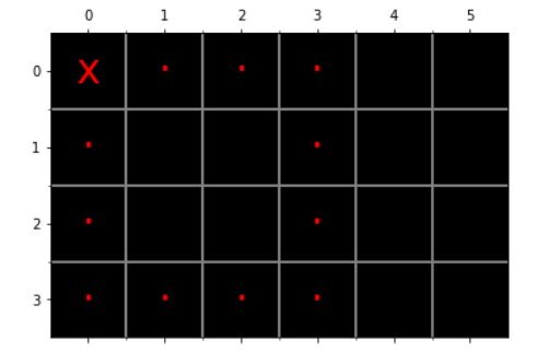
carla.display_world()
## TODO: Move carla around, using your new turn_right() function
## Display the result and the state as it changes
carla = car.Car(initial_position, velocity, world)
for i in range(4):
    for j in range(3):
        carla.move()
    carla.turn_right()
carla.display_world()
重载颜色加法
class Color(object):

    # Initializes a color with rgb values
    def __init__(self, r, g, b):
        self.r = r
        self.g = g
        self.b = b

    # Called when a Color object is printed out
    def __repr__(self):
        '''Display a color swatch and returns a text description of r,g,b values'''

        plt.imshow([[(self.r/255, self.g/255, self.b/255)]])

        return 'r, g, b = ' + str(self.r) + ', ' + str(self.g) + ', ' + str(self.b)


    ## TODO: Complete this add function to add two colors together
    def __add__(self, other):
        '''Adds the r, g, and b components of each color together
           and averaging them.
           The new Color object, with these averaged rgb values,
           is returned.'''
        self.r = self.r + other.r
        self.g = self.g + other.g
        self.b = self.b + other.b
        return self
# Notice we are importing the color class!

import numpy as np
import color

%matplotlib inline

# Auto-reload function so that this notebook keeps up with
# changes in the class file
%load_ext autoreload
%autoreload 2
color1 = color.Color(250, 0, 0)
print(color1)
color2 = color.Color(0,0, 250)
print(color2)
# Add the two colors to create a *new* color object
new_color = color1 + color2
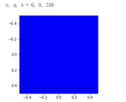
print(new_color)
状态转为为矩阵
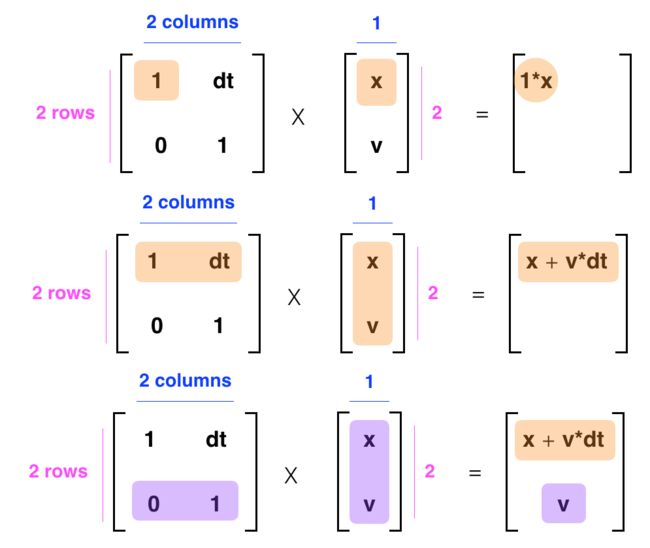
状态向量是一列值,比如我们感兴趣位置X和速度V:
使用状态向量,我们可以在一个矩阵乘法步骤中预测新状态。
矩阵乘法
左边的2*2矩阵通常称为状态变换矩阵
如果x和y不相互依赖,存在单独且恒定的x速度和y速度分量
