hello,大家好,今天我们来分享一个做细胞通讯的分析软件NicheNet,这个软件最大特点就是预测配体活性,所以很多文章里都将NicheNet和cellphoneDB联合使用,从而达到最好的通讯分析效果,文章在NicheNet: modeling intercellular communication by linking ligands to target genes,2019年12月发表于nature methods,影响因子30分,对于这个方法,其实也一直在用,和cellphoneDB联合使用是真的赞,我们先来分享文章,最后分享一下代码。
Abstract
Computational methods that model how gene expression of a cell is influenced by interacting cells are lacking. (我们分析配受体通常只看配受体基因的表达量,真正是否起作用其实需要其他验证)We present NicheNet (https://github.com/saeyslab/nichenetr), a method that predicts ligand–target(看到了没,不是配受体,而是配体靶基因) links between interacting cells by combining their expression data with prior knowledge on signaling and gene regulatory networks. We applied NicheNet to tumor and immune cell microenvironment data and demonstrate that NicheNet can infer active ligands and their gene regulatory effects on interacting cells.(预测配体活性)。
Introduction
我们提炼一下其中的信息。
目前方法的缺点:a functional understanding of cell–cell communication requires knowledge about the influence of these ligand–receptor interactions on target gene expression(通讯导致的影响没有考虑到)。所以,there is a need for computational methodologies that use expression data of interacting cells to infer the effects of sender-cell ligands on receiver-cell expression。
- NicheNet的特点:
1、分析物种:人和小鼠(human or mouse gene expression data)
 图片.png
图片上的内容基本概括了软件的优势,把配体,受体,靶基因联合起来进行分析。
2、NicheNet’s prior model goes beyond ligand–receptor interactions and incorporates intracellular signaling as well.(先验知识更广)。
3、NicheNet can predict which ligands influence the expression in another cell, which target genes are affected by each ligand and which signaling mediators may be involved.(配体和靶基因的相互联系)。
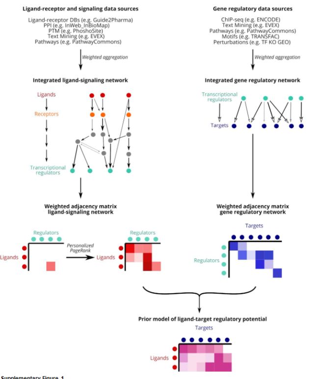
看一看数据库的特点:
The prior model at the basis of NicheNet denotes how strongly existing knowledge supports that a ligand may regulate the expression of a target gene.为了计算配体靶基因的调控潜能,we integrated biological knowledge about ligand-to-target signaling paths as follows:
-
1、we collected multiple complementary data sources covering ligand–receptor, signal transduction and gene regulatory interactions(**我们收集了涵盖配体-受体,信号转导和基因调控相互作用的多个互补数据源 **)
 图片.png
 -
2、Secondly, we integrated these individual data sources into weighted networks(依据先验知识计算权重网络)。关于权重的计算涉及到很深的算法,我们暂时不用管这个
 图片.png
作者为了最大程度改进这个网络,也做了很多的优化,当然,准确度肯定更高。 3、we calculated a regulatory potential score between all pairs of ligands and target genes
这个分数真的让我很头疼,算法有点难。To calculate this, we used network propagation methods on the integrated networks to propagate the signal from a ligand, over receptors, signaling proteins and transcriptional regulators, to end at target genes.
也就是说,真正的通讯过程是配体---受体---信号蛋白---转录调节子(TF)---靶基因,现在明白为什么我们只分析配受体的局限性了吧。
接下来讲了一下用法,根据目标细胞的基因表达特征来判断配体细胞配体的活性排名,最后进行可视化,先验模型也进行了很大程度的优化。
当然这里我们需要注意的一点,我们在预测配体细胞配体活性的时候,需要靶基因,实验不同的靶基因我们往往很难得到,所以一般采用某种细胞类型的差异基因,但这个方法值得商榷,但是一定程度上可以得到一些可靠的结果。
看一看模型优化后的比较
We compared target gene and ligand activity prediction performances of the final optimized model with an unoptimized model and models constructed from random networks

Parameter optimization was performed to maximize both target gene and ligand activity prediction accuracy,这部分对通讯网络优化的检验,当然,效果很好,不好这篇文章就见不到了
接下来是细胞类型对配体分布的无偏估计,当然,效果也不错。
进一步多个方法的比较,当然NicheNet最好

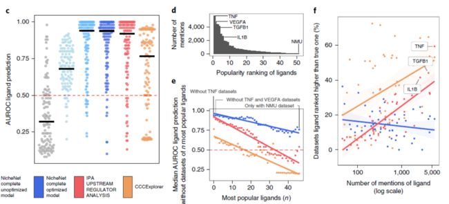
其实 e, Analysis of popularity bias in ligand activity prediction performance by iteratively leaving out datasets of the n most popular ligands.** f, Analysis of popularity bias in the ligand rankings from the ligand activity prediction procedure. The smoothing lines shown in e and f are the result of fitting a linear regression model (n = 51 different ligands). The accompanying shaded region indicates the 95% confidence interval.
关于AUROC我之前分享过,文章在 深入理解R包AUcell对于分析单细胞的作用。
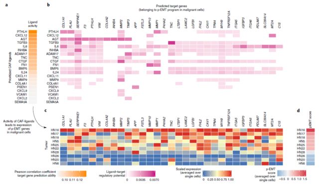
接下来就是一些例子了:
当然,都是基于模型进行预测:
我们看一下示例代码
Prepare NicheNet analysis
Load required packages, read in the Seurat object with processed expression data of interacting cells and NicheNet’s ligand-target prior model, ligand-receptor network and weighted integrated networks
The NicheNet ligand-receptor network and weighted networks are necessary to define and show possible ligand-receptor interactions between two cell populations. The ligand-target matrix denotes the prior potential that particular ligands might regulate the expression of particular target genes. This matrix is necessary to prioritize possible ligand-receptor interactions based on observed gene expression effects (i.e. NicheNet’s ligand activity analysis) and infer affected target genes of these prioritized ligands.
Load Packages:
library(nichenetr)
library(Seurat) # please update to Seurat V4
library(tidyverse)
If you would use and load other packages, we recommend to load these 3 packages after the others.
Read in the expression data of interacting cells:
The dataset used here is publicly available single-cell data from immune cells in the T cell area of the inguinal lymph node. The data was processed and aggregated by applying the Seurat alignment pipeline. The Seurat object contains this aggregated data. Note that this should be a Seurat v3 object and that gene should be named by their official mouse/human gene symbol.
seuratObj = readRDS(url("https://zenodo.org/record/3531889/files/seuratObj.rds"))
[email protected] %>% head()
##         nGene nUMI orig.ident aggregate res.0.6 celltype nCount_RNA nFeature_RNA
## W380370   880 1611      LN_SS        SS       1    CD8 T       1607          876
## W380372   541  891      LN_SS        SS       0    CD4 T        885          536
## W380374   742 1229      LN_SS        SS       0    CD4 T       1223          737
## W380378   847 1546      LN_SS        SS       1    CD8 T       1537          838
## W380379   839 1606      LN_SS        SS       0    CD4 T       1603          836
## W380381   517  844      LN_SS        SS       0    CD4 T        840          513
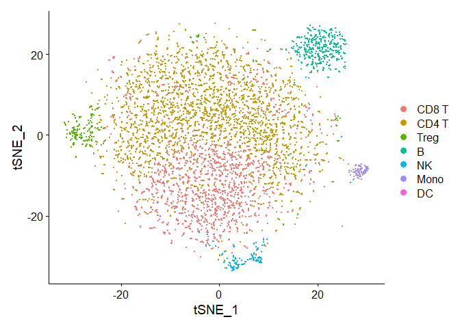
Visualize which cell populations are present: CD4 T cells (including regulatory T cells), CD8 T cells, B cells, NK cells, dendritic cells (DCs) and inflammatory monocytes
[email protected]$celltype %>% table() # note that the number of cells of some cell types is very low and should preferably be higher for a real application
## .
##     B CD4 T CD8 T    DC  Mono    NK  Treg
##   382  2562  1645    18    90   131   199
DimPlot(seuratObj, reduction = "tsne")
Visualize the data to see to which condition cells belong. The metadata dataframe column that denotes the condition (steady-state or after LCMV infection) is here called ‘aggregate.’
[email protected]$aggregate %>% table()
## .
## LCMV   SS
## 3886 1141
DimPlot(seuratObj, reduction = "tsne", group.by = "aggregate")

Read in NicheNet’s ligand-target prior model, ligand-receptor network and weighted integrated networks:
ligand_target_matrix = readRDS(url("https://zenodo.org/record/3260758/files/ligand_target_matrix.rds"))
ligand_target_matrix[1:5,1:5] # target genes in rows, ligands in columns
##                 CXCL1        CXCL2        CXCL3        CXCL5         PPBP
## A1BG     3.534343e-04 4.041324e-04 3.729920e-04 3.080640e-04 2.628388e-04
## A1BG-AS1 1.650894e-04 1.509213e-04 1.583594e-04 1.317253e-04 1.231819e-04
## A1CF     5.787175e-04 4.596295e-04 3.895907e-04 3.293275e-04 3.211944e-04
## A2M      6.027058e-04 5.996617e-04 5.164365e-04 4.517236e-04 4.590521e-04
## A2M-AS1  8.898724e-05 8.243341e-05 7.484018e-05 4.912514e-05 5.120439e-05

lr_network = readRDS(url("https://zenodo.org/record/3260758/files/lr_network.rds"))
head(lr_network)
## # A tibble: 6 x 4
##   from  to    source         database
##
## 1 CXCL1 CXCR2 kegg_cytokines kegg
## 2 CXCL2 CXCR2 kegg_cytokines kegg
## 3 CXCL3 CXCR2 kegg_cytokines kegg
## 4 CXCL5 CXCR2 kegg_cytokines kegg
## 5 PPBP  CXCR2 kegg_cytokines kegg
## 6 CXCL6 CXCR2 kegg_cytokines kegg

weighted_networks = readRDS(url("https://zenodo.org/record/3260758/files/weighted_networks.rds"))
weighted_networks_lr = weighted_networks$lr_sig %>% inner_join(lr_network %>% distinct(from,to), by = c("from","to"))

head(weighted_networks$lr_sig) # interactions and their weights in the ligand-receptor + signaling network
## # A tibble: 6 x 3
##   from  to     weight
##
## 1 A1BG  ABCC6  0.422
## 2 A1BG  ACE2   0.101
## 3 A1BG  ADAM10 0.0970
## 4 A1BG  AGO1   0.0525
## 5 A1BG  AKT1   0.0855
## 6 A1BG  ANXA7  0.457
head(weighted_networks$gr) # interactions and their weights in the gene regulatory network
## # A tibble: 6 x 3
##   from  to     weight
##
## 1 A1BG  A2M    0.0294
## 2 AAAS  GFAP   0.0290
## 3 AADAC CYP3A4 0.0422
## 4 AADAC IRF8   0.0275
## 5 AATF  ATM    0.0330
## 6 AATF  ATR    0.0355
Because the expression data is of mouse origin, we will convert the NicheNet network gene symbols from human to mouse based on one-to-one orthology:
lr_network = lr_network %>% mutate(from = convert_human_to_mouse_symbols(from), to = convert_human_to_mouse_symbols(to)) %>% drop_na()
colnames(ligand_target_matrix) = ligand_target_matrix %>% colnames() %>% convert_human_to_mouse_symbols()
rownames(ligand_target_matrix) = ligand_target_matrix %>% rownames() %>% convert_human_to_mouse_symbols()

ligand_target_matrix = ligand_target_matrix %>% .[!is.na(rownames(ligand_target_matrix)), !is.na(colnames(ligand_target_matrix))]

weighted_networks_lr = weighted_networks_lr %>% mutate(from = convert_human_to_mouse_symbols(from), to = convert_human_to_mouse_symbols(to)) %>% drop_na()
Perform the NicheNet analysis
In this case study, we want to apply NicheNet to predict which ligands expressed by all immune cells in the T cell area of the lymph node are most likely to have induced the differential expression in CD8 T cells after LCMV infection.
As described in the main vignette, the pipeline of a basic NicheNet analysis consist of the following steps:
1. Define a “sender/niche” cell population and a “receiver/target” cell population present in your expression data and determine which genes are expressed in both populations
In this case study, the receiver cell population is the ‘CD8 T’ cell population, whereas the sender cell populations are ‘CD4 T,’ ‘Treg,’ ‘Mono,’ ‘NK,’ ‘B’ and ‘DC.’ We will consider a gene to be expressed when it is expressed in at least 10% of cells in one cluster.
## receiver
receiver = "CD8 T"
expressed_genes_receiver = get_expressed_genes(receiver, seuratObj, pct = 0.10)

background_expressed_genes = expressed_genes_receiver %>% .[. %in% rownames(ligand_target_matrix)]
## sender
sender_celltypes = c("CD4 T","Treg", "Mono", "NK", "B", "DC")

list_expressed_genes_sender = sender_celltypes %>% unique() %>% lapply(get_expressed_genes, seuratObj, 0.10) # lapply to get the expressed genes of every sender cell type separately here
expressed_genes_sender = list_expressed_genes_sender %>% unlist() %>% unique()
2. Define a gene set of interest: these are the genes in the “receiver/target” cell population that are potentially affected by ligands expressed by interacting cells (e.g. genes differentially expressed upon cell-cell interaction)
Here, the gene set of interest are the genes differentially expressed in CD8 T cells after LCMV infection. The condition of interest is thus ‘LCMV,’ whereas the reference/steady-state condition is ‘SS.’ The notion of conditions can be extracted from the metadata column ‘aggregate.’ The method to calculate the differential expression is here the standard Seurat Wilcoxon test, but this can be changed if necessary.
seurat_obj_receiver= subset(seuratObj, idents = receiver)
seurat_obj_receiver = SetIdent(seurat_obj_receiver, value = seurat_obj_receiver[["aggregate"]])

condition_oi = "LCMV"
condition_reference = "SS"

DE_table_receiver = FindMarkers(object = seurat_obj_receiver, ident.1 = condition_oi, ident.2 = condition_reference, min.pct = 0.10) %>% rownames_to_column("gene")

geneset_oi = DE_table_receiver %>% filter(p_val_adj <= 0.05 & abs(avg_log2FC) >= 0.25) %>% pull(gene)
geneset_oi = geneset_oi %>% .[. %in% rownames(ligand_target_matrix)]
3. Define a set of potential ligands: these are ligands that are expressed by the “sender/niche” cell population and bind a (putative) receptor expressed by the “receiver/target” population
Because we combined the expressed genes of each sender cell type, in this example, we will perform one NicheNet analysis by pooling all ligands from all cell types together. Later on during the interpretation of the output, we will check which sender cell type expresses which ligand.
ligands = lr_network %>% pull(from) %>% unique()
receptors = lr_network %>% pull(to) %>% unique()

expressed_ligands = intersect(ligands,expressed_genes_sender)
expressed_receptors = intersect(receptors,expressed_genes_receiver)

potential_ligands = lr_network %>% filter(from %in% expressed_ligands & to %in% expressed_receptors) %>% pull(from) %>% unique()
4) Perform NicheNet ligand activity analysis: rank the potential ligands based on the presence of their target genes in the gene set of interest (compared to the background set of genes)
ligand_activities = predict_ligand_activities(geneset = geneset_oi, background_expressed_genes = background_expressed_genes, ligand_target_matrix = ligand_target_matrix, potential_ligands = potential_ligands)

ligand_activities = ligand_activities %>% arrange(-pearson) %>% mutate(rank = rank(desc(pearson)))
ligand_activities
## # A tibble: 44 x 5
##    test_ligand auroc  aupr pearson  rank
##
##  1 Ebi3        0.638 0.234  0.197      1
##  2 Il15        0.582 0.163  0.0961     2
##  3 Crlf2       0.549 0.163  0.0758     3
##  4 App         0.499 0.141  0.0655     4
##  5 Tgfb1       0.494 0.140  0.0558     5
##  6 Ptprc       0.536 0.149  0.0554     6
##  7 H2-M3       0.525 0.157  0.0528     7
##  8 Icam1       0.543 0.142  0.0486     8
##  9 Cxcl10      0.531 0.141  0.0408     9
## 10 Adam17      0.517 0.137  0.0359    10
## # ... with 34 more rows
The different ligand activity measures (auroc, aupr, pearson correlation coefficient) are a measure for how well a ligand can predict the observed differentially expressed genes compared to the background of expressed genes. In our validation study, we showed that the pearson correlation coefficient between a ligand’s target predictions and the observed transcriptional response was the most informative measure to define ligand activity. Therefore, NicheNet ranks the ligands based on their pearson correlation coefficient. This allows us to prioritize ligands inducing the antiviral response in CD8 T cells.
The number of top-ranked ligands that are further used to predict active target genes and construct an active ligand-receptor network is here 20.
best_upstream_ligands = ligand_activities %>% top_n(20, pearson) %>% arrange(-pearson) %>% pull(test_ligand) %>% unique()
These ligands are expressed by one or more of the input sender cells. To see which cell population expresses which of these top-ranked ligands, you can run the following:
DotPlot(seuratObj, features = best_upstream_ligands %>% rev(), cols = "RdYlBu") + RotatedAxis()

As you can see, most op the top-ranked ligands seem to be mainly expressed by dendritic cells and monocytes.
5) Infer receptors and top-predicted target genes of ligands that are top-ranked in the ligand activity analysis
Active target gene inference
active_ligand_target_links_df = best_upstream_ligands %>% lapply(get_weighted_ligand_target_links,geneset = geneset_oi, ligand_target_matrix = ligand_target_matrix, n = 200) %>% bind_rows() %>% drop_na()

active_ligand_target_links = prepare_ligand_target_visualization(ligand_target_df = active_ligand_target_links_df, ligand_target_matrix = ligand_target_matrix, cutoff = 0.33)

order_ligands = intersect(best_upstream_ligands, colnames(active_ligand_target_links)) %>% rev() %>% make.names()
order_targets = active_ligand_target_links_df$target %>% unique() %>% intersect(rownames(active_ligand_target_links)) %>% make.names()
rownames(active_ligand_target_links) = rownames(active_ligand_target_links) %>% make.names() # make.names() for heatmap visualization of genes like H2-T23
colnames(active_ligand_target_links) = colnames(active_ligand_target_links) %>% make.names() # make.names() for heatmap visualization of genes like H2-T23

vis_ligand_target = active_ligand_target_links[order_targets,order_ligands] %>% t()
p_ligand_target_network = vis_ligand_target %>% make_heatmap_ggplot("Prioritized ligands","Predicted target genes", color = "purple",legend_position = "top", x_axis_position = "top",legend_title = "Regulatory potential")  + theme(axis.text.x = element_text(face = "italic")) + scale_fill_gradient2(low = "whitesmoke",  high = "purple", breaks = c(0,0.0045,0.0090))
p_ligand_target_network

Note that not all ligands from the top 20 are present in this ligand-target heatmap. The left-out ligands are ligands that don’t have target genes with high enough regulatory potential scores. Therefore, they did not survive the used cutoffs. To include them, you can be less stringent in the used cutoffs.
Receptors of top-ranked ligands
lr_network_top = lr_network %>% filter(from %in% best_upstream_ligands & to %in% expressed_receptors) %>% distinct(from,to)
best_upstream_receptors = lr_network_top %>% pull(to) %>% unique()

lr_network_top_df_large = weighted_networks_lr %>% filter(from %in% best_upstream_ligands & to %in% best_upstream_receptors)

lr_network_top_df = lr_network_top_df_large %>% spread("from","weight",fill = 0)
lr_network_top_matrix = lr_network_top_df %>% select(-to) %>% as.matrix() %>% magrittr::set_rownames(lr_network_top_df$to)

dist_receptors = dist(lr_network_top_matrix, method = "binary")
hclust_receptors = hclust(dist_receptors, method = "ward.D2")
order_receptors = hclust_receptors$labels[hclust_receptors$order]

dist_ligands = dist(lr_network_top_matrix %>% t(), method = "binary")
hclust_ligands = hclust(dist_ligands, method = "ward.D2")
order_ligands_receptor = hclust_ligands$labels[hclust_ligands$order]

order_receptors = order_receptors %>% intersect(rownames(lr_network_top_matrix))
order_ligands_receptor = order_ligands_receptor %>% intersect(colnames(lr_network_top_matrix))

vis_ligand_receptor_network = lr_network_top_matrix[order_receptors, order_ligands_receptor]
rownames(vis_ligand_receptor_network) = order_receptors %>% make.names()
colnames(vis_ligand_receptor_network) = order_ligands_receptor %>% make.names()
p_ligand_receptor_network = vis_ligand_receptor_network %>% t() %>% make_heatmap_ggplot("Ligands","Receptors", color = "mediumvioletred", x_axis_position = "top",legend_title = "Prior interaction potential")
p_ligand_receptor_network

Receptors of top-ranked ligands, but after considering only bona fide ligand-receptor interactions documented in literature and publicly available databases
lr_network_strict = lr_network %>% filter(database != "ppi_prediction_go" & database != "ppi_prediction")
ligands_bona_fide = lr_network_strict %>% pull(from) %>% unique()
receptors_bona_fide = lr_network_strict %>% pull(to) %>% unique()

lr_network_top_df_large_strict = lr_network_top_df_large %>% distinct(from,to) %>% inner_join(lr_network_strict, by = c("from","to")) %>% distinct(from,to)
lr_network_top_df_large_strict = lr_network_top_df_large_strict %>% inner_join(lr_network_top_df_large, by = c("from","to"))

lr_network_top_df_strict = lr_network_top_df_large_strict %>% spread("from","weight",fill = 0)
lr_network_top_matrix_strict = lr_network_top_df_strict %>% select(-to) %>% as.matrix() %>% magrittr::set_rownames(lr_network_top_df_strict$to)

dist_receptors = dist(lr_network_top_matrix_strict, method = "binary")
hclust_receptors = hclust(dist_receptors, method = "ward.D2")
order_receptors = hclust_receptors$labels[hclust_receptors$order]

dist_ligands = dist(lr_network_top_matrix_strict %>% t(), method = "binary")
hclust_ligands = hclust(dist_ligands, method = "ward.D2")
order_ligands_receptor = hclust_ligands$labels[hclust_ligands$order]

order_receptors = order_receptors %>% intersect(rownames(lr_network_top_matrix_strict))
order_ligands_receptor = order_ligands_receptor %>% intersect(colnames(lr_network_top_matrix_strict))

vis_ligand_receptor_network_strict = lr_network_top_matrix_strict[order_receptors, order_ligands_receptor]
rownames(vis_ligand_receptor_network_strict) = order_receptors %>% make.names()
colnames(vis_ligand_receptor_network_strict) = order_ligands_receptor %>% make.names()
p_ligand_receptor_network_strict = vis_ligand_receptor_network_strict %>% t() %>% make_heatmap_ggplot("Ligands","Receptors", color = "mediumvioletred", x_axis_position = "top",legend_title = "Prior interaction potential\n(bona fide)")
p_ligand_receptor_network_strict

6) Add log fold change information of ligands from sender cells
In some cases, it might be possible to also check upregulation of ligands in sender cells. This can add a useful extra layer of information next to the ligand activities defined by NicheNet, because you can assume that some of the ligands inducing DE in receiver cells, will be DE themselves in the sender cells.
Here this is possible: we will define the log fold change between LCMV and steady-state in all sender cell types and visualize this as extra information.
# DE analysis for each sender cell type
# this uses a new nichenetr function - reinstall nichenetr if necessary!
DE_table_all = Idents(seuratObj) %>% levels() %>% intersect(sender_celltypes) %>% lapply(get_lfc_celltype, seurat_obj = seuratObj, condition_colname = "aggregate", condition_oi = condition_oi, condition_reference = condition_reference, expression_pct = 0.10) %>% reduce(full_join)
DE_table_all[is.na(DE_table_all)] = 0

# Combine ligand activities with DE information
ligand_activities_de = ligand_activities %>% select(test_ligand, pearson) %>% rename(ligand = test_ligand) %>% left_join(DE_table_all %>% rename(ligand = gene))
ligand_activities_de[is.na(ligand_activities_de)] = 0

# make LFC heatmap
lfc_matrix = ligand_activities_de  %>% select(-ligand, -pearson) %>% as.matrix() %>% magrittr::set_rownames(ligand_activities_de$ligand)
rownames(lfc_matrix) = rownames(lfc_matrix) %>% make.names()

order_ligands = order_ligands[order_ligands %in% rownames(lfc_matrix)]
vis_ligand_lfc = lfc_matrix[order_ligands,]

colnames(vis_ligand_lfc) = vis_ligand_lfc %>% colnames() %>% make.names()

p_ligand_lfc = vis_ligand_lfc %>% make_threecolor_heatmap_ggplot("Prioritized ligands","LFC in Sender", low_color = "midnightblue",mid_color = "white", mid = median(vis_ligand_lfc), high_color = "red",legend_position = "top", x_axis_position = "top", legend_title = "LFC") + theme(axis.text.y = element_text(face = "italic"))
p_ligand_lfc

# change colors a bit to make them more stand out
p_ligand_lfc = p_ligand_lfc + scale_fill_gradientn(colors = c("midnightblue","blue", "grey95", "grey99","firebrick1","red"),values = c(0,0.1,0.2,0.25, 0.40, 0.7,1), limits = c(vis_ligand_lfc %>% min() - 0.1, vis_ligand_lfc %>% max() + 0.1))
p_ligand_lfc

7) Summary visualizations of the NicheNet analysis
For example, you can make a combined heatmap of ligand activities, ligand expression, ligand log fold change and the target genes of the top-ranked ligands. The plots for the log fold change and target genes were already made. Let’s now make the heatmap for ligand activities and for expression.
# ligand activity heatmap
ligand_pearson_matrix = ligand_activities %>% select(pearson) %>% as.matrix() %>% magrittr::set_rownames(ligand_activities$test_ligand)

rownames(ligand_pearson_matrix) = rownames(ligand_pearson_matrix) %>% make.names()
colnames(ligand_pearson_matrix) = colnames(ligand_pearson_matrix) %>% make.names()

vis_ligand_pearson = ligand_pearson_matrix[order_ligands, ] %>% as.matrix(ncol = 1) %>% magrittr::set_colnames("Pearson")
p_ligand_pearson = vis_ligand_pearson %>% make_heatmap_ggplot("Prioritized ligands","Ligand activity", color = "darkorange",legend_position = "top", x_axis_position = "top", legend_title = "Pearson correlation coefficient\ntarget gene prediction ability)") + theme(legend.text = element_text(size = 9))
# ligand expression Seurat dotplot
order_ligands_adapted = order_ligands
order_ligands_adapted[order_ligands_adapted == "H2.M3"] = "H2-M3" # cf required use of make.names for heatmap visualization | this is not necessary if these ligands are not in the list of prioritized ligands!
order_ligands_adapted[order_ligands_adapted == "H2.T23"] = "H2-T23" # cf required use of make.names for heatmap visualization | this is not necessary if these ligands are not in the list of prioritized ligands!
rotated_dotplot = DotPlot(seuratObj %>% subset(celltype %in% sender_celltypes), features = order_ligands_adapted %>% rev(), cols = "RdYlBu") + coord_flip() + theme(legend.text = element_text(size = 10), legend.title = element_text(size = 12)) # flip of coordinates necessary because we want to show ligands in the rows when combining all plots
figures_without_legend = cowplot::plot_grid(
  p_ligand_pearson + theme(legend.position = "none", axis.ticks = element_blank()) + theme(axis.title.x = element_text()),
  rotated_dotplot + theme(legend.position = "none", axis.ticks = element_blank(), axis.title.x = element_text(size = 12), axis.text.y = element_text(face = "italic", size = 9), axis.text.x = element_text(size = 9,  angle = 90,hjust = 0)) + ylab("Expression in Sender") + xlab("") + scale_y_discrete(position = "right"),
  p_ligand_lfc + theme(legend.position = "none", axis.ticks = element_blank()) + theme(axis.title.x = element_text()) + ylab(""),
  p_ligand_target_network + theme(legend.position = "none", axis.ticks = element_blank()) + ylab(""),
  align = "hv",
  nrow = 1,
  rel_widths = c(ncol(vis_ligand_pearson)+6, ncol(vis_ligand_lfc) + 7, ncol(vis_ligand_lfc) + 8, ncol(vis_ligand_target)))

legends = cowplot::plot_grid(
    ggpubr::as_ggplot(ggpubr::get_legend(p_ligand_pearson)),
    ggpubr::as_ggplot(ggpubr::get_legend(rotated_dotplot)),
    ggpubr::as_ggplot(ggpubr::get_legend(p_ligand_lfc)),
    ggpubr::as_ggplot(ggpubr::get_legend(p_ligand_target_network)),
    nrow = 1,
    align = "h", rel_widths = c(1.5, 1, 1, 1))

combined_plot = cowplot::plot_grid(figures_without_legend, legends, rel_heights = c(10,5), nrow = 2, align = "hv")
combined_plot

生活很好,有你更好