简介
本文要介绍的是由浙江大学联合新加坡国立大学提出的AFM模型。通过名字也可以看出,此模型又是基于FM模型的改进,其中A代表”Attention“,即AFM模型实际上是在FM模型中引入了注意力机制改进得来的。之所以要在FM模型中引入注意力机制,是因为传统的FM模型对所有的交叉特征都平等对待,即每个交叉特征的权重都是相同的(都为1)。而在实际应用中,不同交叉特征的重要程度往往是不一样的。如果”一视同仁“地对待所有的交叉特征,不考虑不同特征对结果的影响程度,事实上消解了大量有价值的信息。
关于FM模型,可以参考推荐系统之FM(因子分解机)模型原理以及代码实践。
推荐系统中的注意力机制
这里再举个例子,说明一下注意力机制是如何在推荐系统中派上用场的。注意力机制基于假设——不同的交叉特征对结果的影响程度不同,以更直观的业务场景为例,用户对不同交叉特征的关注程度应该是不同的。举例来说,如果应用场景是预测一位男性用户是否会购买一款键盘的可能性,那么”性别=男”和“购买历史包含鼠标“这一交叉特征,很可能比”性别=男”和“年龄=30“这一交叉特征重要,模型应该投入更多的”注意力“在前面的特征上。正因如此,将注意力机制引入推荐系统中也显得理所当然了。
模型
在介绍AFM模型之前,先给出FM模型的方程:

Pair-wise 交互层
Pair-wise 交互层将个向量扩展到个交叉向量,每个交叉向量都是通过对两个不同的向量进行内积来计算的。可以通过以下公式来描述:


这里其实跟NFM模型的核心操作类似,具体可以参考推荐系统之NFM模型原理以及代码实践。
Attention-based Pooling层
下面看一下作者是如何将注意力机制加入到FM模型中去的。其实也很简单,只是在上述的交叉特征项前加入了注意力分数权重,具体如下:

其中 就是交叉特征 的注意力分数,它可以被看做是在预测过程中 的重要程度。
为了估计 ,一个很自然的想法就是通过直接最小化目标损失函数来估计,在技术上似乎也是可行的。但是,对于从未在训练集中出现的共同出现过的特征,那么意味着 ,故对应的注意力分数 不可能通过估计得到。
为了解决这个问题,作者提出了通过MLP来参数化注意力分数,作者称之为”注意力网络“,其定义如下:
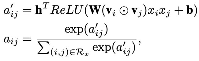
直观来看,注意力网络就是将交叉特征首先通过一个全连接层,接着通过Relu激活函数,再乘以权重参数得到,接着再通过一个Softmax层,将其映射成注意力权重,此时有。
AFM模型
下面给出完整的AFM框架图:


代码实践
模型部分:
import torch
import torch.nn as nn
from BaseModel.basemodel import BaseModel

class AFM(BaseModel):
    def __init__(self, config, dense_features_cols, sparse_features_cols):
        super(AFM, self).__init__(config)
        self.num_fields = config['num_fields']
        self.embed_dim = config['embed_dim']
        self.l2_reg_w = config['l2_reg_w']

        # 稠密和稀疏特征的数量
        self.num_dense_feature = dense_features_cols.__len__()
        self.num_sparse_feature = sparse_features_cols.__len__()

        # AFM的线性部分,对应 ∑W_i*X_i, 这里包含了稠密和稀疏特征
        self.linear_model = nn.Linear(self.num_dense_feature + self.num_sparse_feature, 1)

        # AFM的Embedding层,只是针对稀疏特征,有待改进。
        self.embedding_layers = nn.ModuleList([
            nn.Embedding(num_embeddings=feat_dim, embedding_dim=config['embed_dim'])
                for feat_dim in sparse_features_cols
        ])

        # Attention Network
        self.attention = torch.nn.Linear(self.embed_dim, self.embed_dim, bias=True)
        self.projection = torch.nn.Linear(self.embed_dim, 1, bias=False)
        self.attention_dropout = nn.Dropout(config['dropout_rate'])

        # prediction layer
        self.predict_layer = torch.nn.Linear(self.embed_dim, 1)

    def forward(self, x):
        # 先区分出稀疏特征和稠密特征,这里是按照列来划分的,即所有的行都要进行筛选
        dense_input, sparse_inputs = x[:, :self.num_dense_feature], x[:, self.num_dense_feature:]
        sparse_inputs = sparse_inputs.long()

        # 求出线性部分
        linear_logit = self.linear_model(x)

        # 求出稀疏特征的embedding向量
        sparse_embeds = [self.embedding_layers[i](sparse_inputs[:, i]) for i in range(sparse_inputs.shape[1])]
        sparse_embeds = torch.cat(sparse_embeds, axis=-1)
        sparse_embeds = sparse_embeds.view(-1, self.num_sparse_feature, self.embed_dim)

        # calculate inner product
        row, col = list(), list()
        for i in range(self.num_fields - 1):
            for j in range(i + 1, self.num_fields):
                row.append(i), col.append(j)
        p, q = sparse_embeds[:, row], sparse_embeds[:, col]
        inner_product = p * q

        # 通过Attention network得到注意力分数
        attention_scores = torch.relu(self.attention(inner_product))
        attention_scores = torch.softmax(self.projection(attention_scores), dim=1)

        # dim=1 按行求和
        attention_output = torch.sum(attention_scores * inner_product, dim=1)
        attention_output = self.attention_dropout(attention_output)

        # Prodict Layer
        # for regression problem with MSELoss
        y_pred = self.predict_layer(attention_output) + linear_logit
        # for classifier problem with LogLoss
        # y_pred = torch.sigmoid(y_pred)
        return y_pred
在criteo数据集上测试,测试代码如下:
import torch
from AFM.network import AFM
from DeepCrossing.trainer import Trainer
import torch.utils.data as Data
from Utils.criteo_loader import getTestData, getTrainData
afm_config = \
{
'num_fields': 26, # 这里配置的只是稀疏特征的个数
'embed_dim': 8, # 用于控制稀疏特征经过Embedding层后的稠密特征大小
'seed': 1024,
'l2_reg_w': 0.001,
'dropout_rate': 0.1,
'num_epoch': 200,
'batch_size': 64,
'lr': 1e-3,
'l2_regularization': 1e-4,
'device_id': 0,
'use_cuda': False,
'train_file': '../Data/criteo/processed_data/train_set.csv',
'fea_file': '../Data/criteo/processed_data/fea_col.npy',
'validate_file': '../Data/criteo/processed_data/val_set.csv',
'test_file': '../Data/criteo/processed_data/test_set.csv',
'model_name': '../TrainedModels/AFM.model'
}
if __name__ == "__main__":
####################################################################################
# AFM 模型
####################################################################################
training_data, training_label, dense_features_col, sparse_features_col = getTrainData(afm_config['train_file'], afm_config['fea_file'])
train_dataset = Data.TensorDataset(torch.tensor(training_data).float(), torch.tensor(training_label).float())
test_data = getTestData(afm_config['test_file'])
test_dataset = Data.TensorDataset(torch.tensor(test_data).float())
afm = AFM(afm_config, dense_features_cols=dense_features_col, sparse_features_cols=sparse_features_col)
####################################################################################
# 模型训练阶段
####################################################################################
# # 实例化模型训练器
trainer = Trainer(model=afm, config=afm_config)
# 训练
trainer.train(train_dataset)
# 保存模型
trainer.save()
####################################################################################
# 模型测试阶段
####################################################################################
afm.eval()
if afm_config['use_cuda']:
afm.loadModel(map_location=lambda storage, loc: storage.cuda(afm_config['device_id']))
afm = afm.cuda()
else:
afm.loadModel(map_location=torch.device('cpu'))
y_pred_probs = afm(torch.tensor(test_data).float())
y_pred = torch.where(y_pred_probs>0.5, torch.ones_like(y_pred_probs), torch.zeros_like(y_pred_probs))
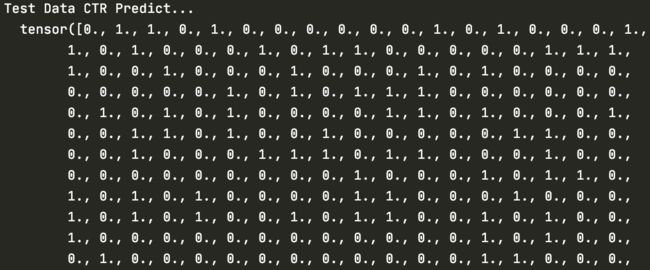
print("Test Data CTR Predict...\n ", y_pred.view(-1))
完整代码见:https://github.com/HeartbreakSurvivor/RsAlgorithms/tree/main/AFM。
参考
- 《深度学习推荐系统》-- 王喆
- Attentional Factorization Machines: Learning the Weight of Feature Interactions via Attention Networks
- https://github.com/shenweichen/DeepCTR-Torch/blob/e7d52151ed3c8beafeda941051aecc6294a4a20d/deepctr_torch/layers/interaction.py#L250
- https://www.cnblogs.com/sunupo/p/12862852.html