【计算机视觉】多视图几何使用OpenCV(Python)进行仿射变换

开始打江山啦，打江山啦，朕的江山从这里开始。

import numpy as np
import cv2
import matplotlib
from matplotlib import pyplot as plt

filename = 'tilef.jpg'
img = cv2.imread(filename)

plt.imshow(img ,cmap = 'gray')

plt.show()

随朕出征，一起征服星辰大海吧！

《CV中的多视图几何》——基础章节

获取图像中的坐标点并打印出来

我们可以看到，如果我们希望获取信息的点在图像中有十字标。

[(37.4032258064516, 96.33870967741936), 
 (263.2096774193548, 178.59677419354836), 
 (329.33870967741933, 52.79032258064518), 
 (155.9516129032258, 6.016129032258107)]

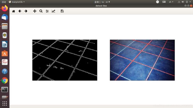
霍夫变化原理

与笛卡尔坐标相对应，我们建立霍夫坐标系，横坐标为斜率，纵坐标为截距。
记住最重要的一点，笛卡尔坐标空间的一点映射到霍夫坐标系是一条直线，笛卡尔坐标系下的一条直线映射到霍夫坐标系下就是一个点。

如果笛卡尔坐标系下确定了两个点，他们可以连接成一直线，在霍夫空间则为两条相交的直线。在霍夫空间通过一点的直线越多，证明在笛卡尔空间里，有越多的点实在一条直线上。

我们OpenCV里面用到的是

cv2.HoughLines(edges, 1, np.pi/180,200)

• 第一个参数是输入图像，且必须是二值图像，在进行霍夫变换之前需要采用阈值法的边缘检测；
• 第二和第三个参数分别是r,θ对应的精度；
• 第四个参数是阈值，判定为直线投票数的最小值；注意，投票数取决于直线上点的个数，因此这个阈值代表了检测到的直线的最短长度。

# find lines in an image by using the Hough transform
#change our image into gray one
gray = cv2.cvtColor(img1,cv2.COLOR_BGR2GRAY)
edges = cv2.Canny(gray,50,200)
plt.figure("detect line")
plt.subplot(121),plt.imshow(edges,'gray')
plt.xticks([]),plt.yticks([])
# hough transform
lines = cv2.HoughLines(edges,1,np.pi/180,160)
# 返回值中的每一个元素都是一对浮点数，表示检测到的直线参数（\rho,\theta）
# 其类型为np.ndarray
lines1 = lines[:,0,:]
#提取为为二维
for rho,theta in lines1[:]: 
	a = np.cos(theta)
	b = np.sin(theta)
	x0 = a*rho
	y0 = b*rho
	x1 = int(x0 + 1000*(-b))
	y1 = int(y0 + 1000*(a))
	x2 = int(x0 - 1000*(-b))
	y2 = int(y0 - 1000*(a)) 
	cv2.line(img1,(x1,y1),(x2,y2),(255,0,0),1)

plt.subplot(122),plt.imshow(img1,)
plt.xticks([]),plt.yticks([])
plt.show()

仿射变换

仿射变换是指图像可以通过一系列的几何变化来实现平移，旋转等，保持图像的平直性和平行性。（直线仍是直线，平行线仍是平行线）

为了得到仿射变换的4points，我们需要转换一下数据类型。我们先来探索一下：

>>> import numpy as np
>>> list=[(38.81034308370755, 94.5354816523041), (263.86192701379616, 177.25992232067), (329.6304264271554, 50.34727110895335), (156.98811546708743, 5.645244163935786)]
>>> list
[(38.81034308370755, 94.5354816523041), (263.86192701379616, 177.25992232067), (329.6304264271554, 50.34727110895335), (156.98811546708743, 5.645244163935786)]
>>> list[1]
(263.86192701379616, 177.25992232067)
>>> list[0]
(38.81034308370755, 94.5354816523041)
>>> list[1].tpye
Traceback (most recent call last):
  File "", line 1, in <module>
AttributeError: 'tuple' object has no attribute 'tpye'
>>> list[1].type
Traceback (most recent call last):
  File "", line 1, in <module>
AttributeError: 'tuple' object has no attribute 'type'
>>> pst1=np.float32(list)
>>> pst1
array([[ 38.810345,  94.535484],
       [263.86194 , 177.25992 ],
       [329.63043 ,  50.34727 ],
       [156.98811 ,   5.645244]], dtype=float32)
>>> pst1.type
Traceback (most recent call last):
  File "", line 1, in <module>
AttributeError: 'numpy.ndarray' object has no attribute 'type'
>>> pts2 = np.float32([[0,0], [360,0], [0,420], [360,420]])
>>> pts2
array([[  0.,   0.],
       [360.,   0.],
       [  0., 420.],
       [360., 420.]], dtype=float32)

按照上述方法在程序运行后打印出我们的两组点坐标。

$ python lab1.py
[[ 34.98387   95.53226 ]
 [261.59677  179.40323 ]
 [328.53226   50.370968]
 [154.33871    5.209677]]
[[  0.   0.]
 [254.   0.]
 [  0. 400.]
 [254. 400.]]

把我们检测到的点和霍夫变换直线检测都显示在窗口上

#we would like to display our points
cv2.circle(img1,(points1[0][0],points1[0][1]),5,(0,0,255),cv2.FILLED)
cv2.circle(img1,(points1[1][0],points1[1][1]),5,(0,255,0),cv2.FILLED)
cv2.circle(img1,(points1[2][0],points1[2][1]),5,(255,0,0),cv2.FILLED)
cv2.circle(img1,(points1[3][0],points1[3][1]),5,(0,0,0),cv2.FILLED)
cv2.imshow('original_images with detected points',img1)
cv2.waitKey(0)

代码过于重复,更换成for循环

for i in range(0,4):
	cv2.circle(...)

我们先尝试一个很简答的方法来看看效果，油管上的小例子：如何截取一个图片中的扑克牌？（翻一翻）

M=cv2.getPerspectiveTransform(points1,points2)
dst=cv2.warpPerspective(img1,M,(img_width,img_height))
cv2.imshow("img1",img1)
cv2.imshow("dst",dst)
cv2.waitKey(0)

我们看到结果并不是太好。

如何得到H矩阵

这么写真的太傻了。

A=np.array([[pts1[0][0],pts1[0][1],1,0,0,0,-pts2[0][0]*pts1[0][0],-pts2[0][0]*pts1[0][1],-pts2[0][0]],
            [0,0,0,pts1[0][0],pts1[0][1],1,-pts2[0][1]*pts1[0][0],-pts2[0][1]*pts1[0][1],-pts2[0][1]],
	    [pts1[1][0],pts1[1][1],1,0,0,0,-pts2[1][0]*pts1[1][0],-pts2[1][0]*pts1[1][1],-pts2[1][0]],
            [0,0,0,pts1[1][0],pts1[1][1],1,-pts2[1][1]*pts1[1][0],-pts2[1][1]*pts1[1][1],-pts2[1][1]],
	    [pts1[2][0],pts1[2][1],1,0,0,0,-pts2[2][0]*pts1[2][0],-pts2[2][0]*pts1[2][1],-pts2[2][0]],
            [0,0,0,pts1[2][0],pts1[2][1],1,-pts2[2][1]*pts1[2][0],-pts2[2][1]*pts1[2][1],-pts2[2][1]],
            [pts1[3][0],pts1[3][1],1,0,0,0,-pts2[3][0]*pts1[3][0],-pts2[3][0]*pts1[3][1],-pts2[3][0]],
            [0,0,0,pts1[3][0],pts1[3][1],1,-pts2[3][1]*pts1[3][0],-pts2[3][1]*pts1[3][1],-pts2[3][1]]])

这纯属于思考认知错误。

#we would like to display our points
for i in range(0,4):
	cv2.circle(img1,(pts1[i][0],pts1[i][1]),5,(0,0,255),cv2.FILLED)
cv2.imshow('original_images with detected points',img1)
cv2.waitKey(0)
#How to estimate the matrix H?
M=cv2.getPerspectiveTransform(pts1,pts2)



dst=cv2.warpPerspective(img1,M,(img_width,img_height))
cv2.imshow("img1",img1)
cv2.imshow("dst",dst)
cv2.waitKey(0)

还原平直线

第一次的想法是自己重新找点，这有些问题。

print('\n-------- Task 2: Metric rectification --------')
print('Task 2.1: transform 4 chosen points from projective image to affine image')
plt.figure('Please choose 4 points')
plt.imshow(affine_img)
y = plt.ginput(4)
plt.show()
print(y)
pts3=np.array(y)
pts3_homo = np.concatenate((pts3, np.ones((4, 1))), axis=1)  # convert chosen pts to homogeneous coordinate
a1 = pts3_homo[0,:]
b1 = pts3_homo[1,:]
c1 = pts3_homo[2,:]
d1 = pts3_homo[3,:]

aff_hor_0 = np.cross(a1,d1)# image of first horizontal line on affine plane
aff_hor_1 = np.cross(b1,c1)# image of 2nd horizontal line on affine plane

aff_ver_0 = np.cross(a1,b1)# image of first vertical line on affine plane
aff_ver_1 = np.cross(c1,d1)# image of 2nd vertical line on affine plane

c00=np.dot(aff_hor_0[0],aff_ver_0[0])
c01=np.dot(aff_hor_0[0],aff_ver_0[1])+np.dot(aff_hor_0[1],aff_ver_0[0])
c02=np.dot(aff_hor_0[1],aff_ver_0[1])
C0 = np.hstack([c00,c01,c02])
c10=np.dot(aff_hor_1[0],aff_ver_1[0])
c11=np.dot(aff_hor_1[0],aff_ver_1[1])+np.dot(aff_hor_1[1],aff_ver_1[0])
c12=np.dot(aff_hor_1[1],aff_ver_1[1])
C1 = np.hstack([c10,c11,c12])
C = np.vstack([C0,C1])