吴恩达机器学习编程作业ex8 Part1 Anomaly Detection

一、程序及函数

1.引导脚本ex8.m

%% Machine Learning Online Class
%  Exercise 8 | Anomaly Detection and Collaborative Filtering
%
%  Instructions
%  --------------------------------------------------------------
%
%  This file contains code that helps you get started on the
%  exercise. You will need to complete the following functions:
%
%     estimateGaussian.m
%     selectThreshold.m
%     cofiCostFunc.m
%
%  For this exercise, you will not need to change any code in this file,
%  or any other files other than those mentioned above.

%% Initialization
clear;
close all;
clc

%% ================== Part 1: Load Example Dataset  ===================
%  We start this exercise by using a small dataset that is easy to
%  visualize.
%
%  Our example case consists of 2 network server statistics across
%  several machines: the latency and throughput of each machine.
%  This exercise will help us find possibly faulty (or very fast) machines.
%

fprintf('Visualizing example dataset for outlier detection.\n\n');

%  The following command loads the dataset. You should now have the
%  variables X, Xval, yval in your environment
load('ex8data1.mat');

%  Visualize the example dataset
plot(X(:, 1), X(:, 2), 'bx');
axis([0 30 0 30]);
xlabel('Latency (ms)');
ylabel('Throughput (mb/s)');

fprintf('Program paused. Press enter to continue.\n');
pause

%% ================== Part 2: Estimate the dataset statistics ===================
%  For this exercise, we assume a Gaussian distribution for the dataset.
%
%  We first estimate the parameters of our assumed Gaussian distribution, 
%  then compute the probabilities for each of the points and then visualize 
%  both the overall distribution and where each of the points falls in 
%  terms of that distribution.

fprintf('Visualizing Gaussian fit.\n\n');

%  Estimate mu and sigma2
[mu sigma2] = estimateGaussian(X);

%  Returns the density of the multivariate normal at each data point (row) 
%  of X
p = multivariateGaussian(X, mu, sigma2);

%  Visualize the fit
visualizeFit(X,  mu, sigma2);
xlabel('Latency (ms)');
ylabel('Throughput (mb/s)');

fprintf('Program paused. Press enter to continue.\n');
pause;

%% ================== Part 3: Find Outliers ===================
%  Now you will find a good epsilon threshold using a cross-validation set
%  probabilities given the estimated Gaussian distribution

pval = multivariateGaussian(Xval, mu, sigma2);

[epsilon F1] = selectThreshold(yval, pval);
fprintf('Best epsilon found using cross-validation: %e\n', epsilon);
fprintf('Best F1 on Cross Validation Set:  %f\n', F1);
fprintf('   (you should see a value epsilon of about 8.99e-05)\n');
fprintf('   (you should see a Best F1 value of  0.875000)\n\n');

%  Find the outliers in the training set and plot the
outliers = find(p < epsilon);

%  Draw a red circle around those outliers
hold on
plot(X(outliers, 1), X(outliers, 2), 'ro', 'LineWidth', 2, 'MarkerSize', 10);
hold off

fprintf('Program paused. Press enter to continue.\n');
pause;

%% ================== Part 4: Multidimensional Outliers ===================
%  We will now use the code from the previous part and apply it to a 
%  harder problem in which more features describe each datapoint and only 
%  some features indicate whether a point is an outlier.

%  Loads the second dataset. You should now have the
%  variables X, Xval, yval in your environment
load('ex8data2.mat');

%  Apply the same steps to the larger dataset
[mu sigma2] = estimateGaussian(X);

%  Training set 
p = multivariateGaussian(X, mu, sigma2);

%  Cross-validation set
pval = multivariateGaussian(Xval, mu, sigma2);

%  Find the best threshold
[epsilon F1] = selectThreshold(yval, pval);

fprintf('Best epsilon found using cross-validation: %e\n', epsilon);
fprintf('Best F1 on Cross Validation Set:  %f\n', F1);
fprintf('   (you should see a value epsilon of about 1.38e-18)\n');
fprintf('   (you should see a Best F1 value of 0.615385)\n');
fprintf('# Outliers found: %d\n\n', sum(p < epsilon));

2.estimateGaussian.m
mu和sigma的参数估计。

function [mu, sigma2] = estimateGaussian(X)
%ESTIMATEGAUSSIAN This function estimates the parameters of a 
%Gaussian distribution using the data in X
%   [mu sigma2] = estimateGaussian(X), 
%   The input X is the dataset with each n-dimensional data point in one row
%   The output is an n-dimensional vector mu, the mean of the data set
%   and the variances sigma^2, an n x 1 vector

% Useful variables
[m, n] = size(X);

% You should return these values correctly
mu = zeros(n, 1);
sigma2 = zeros(n, 1);

% ====================== YOUR CODE HERE ======================
% Instructions: Compute the mean of the data and the variances
%               In particular, mu(i) should contain the mean of
%               the data for the i-th feature and sigma2(i)
%               should contain variance of the i-th feature.

for i = 1 : n
    mu(i) = mean(X(:,i));
    sigma2(i) = 1 / m * sum( (X(:,i) - mu(i)).^2 );
end
% =============================================================

end

3.selectThreshold.m
通过计算每个epsilon下的F-score去寻找最优的epsilon值，该值将作为选取离群点的阈值。

function [bestEpsilon bestF1] = selectThreshold(yval, pval)
%SELECTTHRESHOLD Find the best threshold (epsilon) to use for selecting
%outliers
%   [bestEpsilon bestF1] = SELECTTHRESHOLD(yval, pval) finds the best
%   threshold to use for selecting outliers based on the results from a
%   validation set (pval) and the ground truth (yval).

bestEpsilon = 0;
bestF1 = 0;
F1 = 0;

stepsize = (max(pval) - min(pval)) / 1000;
for epsilon = min(pval):stepsize:max(pval)
    
    % ====================== YOUR CODE HERE ======================
    % Instructions: Compute the F1 score of choosing epsilon as the
    %               threshold and place the value in F1. The code at the
    %               end of the loop will compare the F1 score for this
    %               choice of epsilon and set it to be the best epsilon if
    %               it is better than the current choice of epsilon.
    %               
    % Note: You can use predictions = (pval < epsilon) to get a binary vector
    %       of 0's and 1's of the outlier predictions
    
    % 求出阈值为epsilon时的预测情况，pval值小于epsilon的点是异常点
    % predictions是一个01列向量
    predictions = (pval < epsilon);
    % 下求F-score
    % 求true positive值
    tp = sum( (predictions == 1) & (yval == 1) );
    % 求false positive值
    fp = sum( (predictions == 1) & (yval == 0) );
    % 求false negative值
    fn = sum( (predictions == 0) & (yval == 1) );
    % 求精准率（precision）
    prec = tp / ( tp + fp );
    % 求召回率（recall）
    rec = tp / ( tp + fn );
    % 最后求F-score
    F1 = 2 * prec * rec / ( prec + rec);
    % F-score越大越好
    % 若当前epsilon对应的F-score更大，则该epsilon是更好的epsilon值
    if F1 > bestF1
       bestF1 = F1;
       bestEpsilon = epsilon;
    end
end

end

二、运行结果

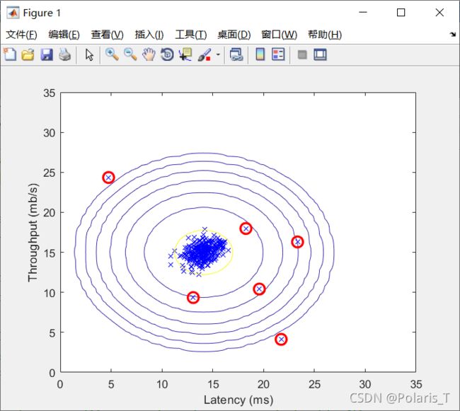
1.二维样本的离群点检测结果示意图：

2.将该算法应用到1000个11维数据样本上进行异常检测，最后发现有117个离群点：