【论文复现】EfficientNet-V1（2020）

前言

原论文地址： https://arxiv.org/abs/1905.11946.

本博客有参考:

太阳花的小绿豆: EfficientNet网络详解.

bilibili: 使用Pytorch搭建EfficientNet网络.

一、背景

\quad 从2012年AlexNet网络的提出开始，卷积神经网络在计算机视觉领域已经发展了9年了。在这过程中先后提出了很多的网络模型，LeNet->AlexNet->VGG->GoogleNet->ResNet->SENet…，这些网络有一个共同点，那就是它们都是一些手工设计的网络。在复现这些网络代码的时候，你可能常常会有这些问题：为什么网络的输入的图像分辨率要固定为224x224？为什么卷积的个数要设置为这个值？为什么网络的深度要是这么大？这些问题你要问设计作者的话，估计回复就四个字——工程经验。真的只能靠经验？真的只能靠玄学？当然不是，那么这篇论文就是来探讨网络的深度、宽度、输入图像的分辨率分别对网络的影响以及它们之间又有着怎样联系。

二、论文思想

2.1、理论和实验上

\quad 在之前的一些论文中，通常会调整宽度width、深度depth、输入图像分辨率resolution其中的一个，来进行手工的调优。有些会在baseline网络如图(a)增加width即增减卷据核的个数（增加feature map的channel）来提升网络的性能如图(b)所示；有些会在baseline网络如图(a)增加depth即使用更多的层结构来提升网络的性能如图©所示；有些会在baseline网络如图(a)增加输入图片的分辨率resolution来提升网络的性能如图(d)所示；但是我们都知道深度、宽度和分辨率是绝对不可能是相互独立的关系，而是相互依赖的，所以本篇论文中会同时增加网络的width、网络的深度depth以及输入网络的分辨率resolution来提升网络的性能如图(e)所示：

• 根据以往的直观经验，增加网络的深度能够得到更加丰富、复杂的feature map，而且能够很好的应用到其它任务中。但网络的深度过深会面临梯度消失，训练困难的问题。
  The intuition is that deeper ConvNet can capture richer and more complex features, and generalize well on new tasks. However, deeper networks are also more difficult to train due to the vanishing gradient problem
• 增加网络的width能够获得更高细粒度的特征并且也更容易训练，但对于width很大而深度较浅的网络往往很难学习到更深层次的特征。
  wider networks tend to be able to capture more fine-grained features and are easier to train. However, extremely wide but shallow networks tend to have difficulties in capturing higher level features.
• 增加输入网络的图像分辨率能够潜在得获得更高细粒度的特征模板，但对于非常高的输入分辨率，准确率的增益也会减小。并且大分辨率图像会增加计算量。
  With higher resolution input images, ConvNets can potentially capture more fine-grained patterns. but the accuracy gain diminishes for very high resolutions.

\quad 下图显示在基准baseline（EfficientNetB-0）上分别增加Width、Depth以及resolution后得到的统计结果。可以看出在增加单个元素的时候，Accuracy大约增加到80%就结束了。

结论一、scaling 宽度width、深度depth、输入图像分辨率resolution的任一个维度，都可以增加accuracy，但是但是增加到一定程度又会趋于稳定。

\quad 接着作者又做了一个实验，如下图，采用不同的d , r 组合，然后不断改变网络的width就得到了如下图所示的4条曲线，通过分析可以发现在相同的FLOPs下，同时增加d 和r 的效果最好。(蓝色表示depth、resolution不变，改变width； 绿色表示resolution不变，$depth=2\ast depth$ 情况下改变width；黄色表示depth不变，$resolution=1.3\ast resolution$ 情况下改变width；红色表示$depth=2\ast depth$，$resolution=1.3\ast resolution$ 情况下改变width)

结论二、scaling 宽度width、深度depth、输入图像分辨率resolution的过程中平衡这三个维度非常重要。

2.2、进一步公式探讨

为了探讨这个问题，作者首先对整个网络进行了抽象：
$$N(d,w,r)=\underset{i=1\dots s}{⨀}{F}_i^{Li}(X_{⟨H_i,W_i,C_i⟩})$$

其中：

• $\underset{i=1\dots s}{⨀}$表示连乘运算
• $F_i$表示一个运算操作，$F_i^{Li}$表示$F_i$运算在$Stag{e}_i$中的执行次数，$Li$是执行次数也是深度depth
• X表示输入$Stag{e}_i$的特征矩阵(input tensor)。$⟨H_i,W_i,C_i⟩$表示X的高度宽度（分辨率resolution）以及Channels(width)

为了探究$d,w,r$这三个因子对最终准确率的影响，则将$d,w,r$加入到公式中，我们可以得到抽象化后的优化问题（在指定资源限制下），其中$s.t.$代表限制条件：

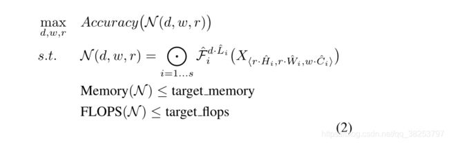
其中：

• $d$用来缩放深度$L_i$
• $r$用来缩放分辨率即影响$H_i$和$\widehat{W_i}
• $w$用来缩放特征矩阵的channel即影响$C_i$
• target_memory为memory限制
• target_flops为FLOPs限制

因为前面说到了网络的深度、宽度、输入分辨率这三个维度其实并不是相互独立的，它们之间是相互依赖的，所以探究d，w，r的关系其实是很复杂的。接着这里作者提出了一种新型的复合型模型缩放方法（Compound Modle Scaling）。

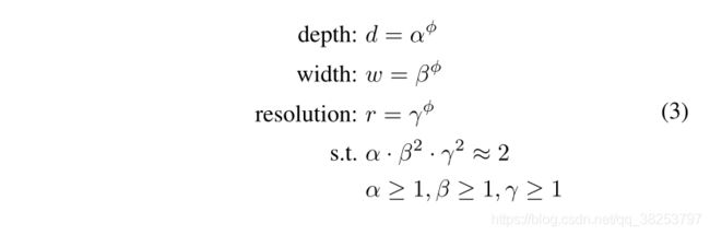
作者是思路是一个卷积网络所有的卷积层必须通过相同的比例常数进行统一扩展，这句话的意思是，三个参数乘上常熟倍率。所以个一个模型的扩展问题，就用数学语言描述为：

注意：

• 某一层的FLOPs计算方法：$featur{e}_w$ x $featur{e}_h$ x $featur{e}_c$ x $kerne{l}_w$ x $kerne{l}_h$ x $kerne{l}_{number}$
• FLOPs（理论计算量）与depth的关系是：当depth翻倍， FLOPs也翻倍
• FLOPs（理论计算量）与width的关系是：当width翻倍（即channal翻倍），FLOPs会翻4倍。当width翻倍，输入特征矩阵的channels和输出特征矩阵的channels或卷积核的个数都会翻倍，所以FLOPs会翻4倍
• FLOPs（理论计算量）与resolution的关系是：当resolution翻倍，FLOPs也会翻4倍，和上面类似因为特征矩阵的宽度和特征矩阵的高度都会翻倍。

所以总的FLOPs倍率可以用近似用$(\alpha .{\beta }^2.{\gamma }^2)$来表示，当限制 $\alpha .{\beta }^2.{\gamma }^2\approx 2$时，对任意的 $\varphi$而言FLOPs相当增加了$2^{\varphi }$倍。

三、EfficientNet-v1网络结构

EfficientNet-B0的网络结构

其中MBConv结构为：

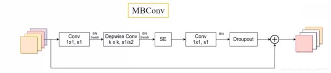
[1x1升维] -> DW -> SE -> 1x1[降维] -> Droupout -> Shortcut

SE模块为：

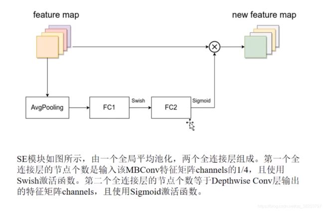
几点细节：

• 第一个1x1卷积升维后，输出的特征矩阵channel是输入特征矩阵channel的n倍，而这个n对应的就是Tabel1中的MBConv后面接的数字，当n为1时，实际上是没用这个1x1卷积的（不需要升维）。
• 第一个1x1卷积、DW后面都是接BN + Swish，而最后的1x1降维卷积是没用激活函数的，要用Identity函数。
• 这里的Droupout用的是Drop path，而不是传统的Dropout。
• 关于shortcut连接，当且仅当输入MBConv结构的特征矩阵和输出的特征矩阵的shape相同且DW卷积的stride=1时才使用。

关于EfficientNet的其他版本，详情请看这张表：

四、PyTorch复现

import torch.nn as nn
from typing import Optional, Callable
from torch import Tensor
from torch.nn import functional as F
from collections import OrderedDict
from functools import partial
import math
import copy
import torch


def _make_divisible(ch, divisor=8, min_ch=None):
    """
    将ch调整到最近的8的倍数
    This function is taken from the original tf repo.
    It ensures that all layers have a channel number that is divisible by 8
    It can be seen here:
    https://github.com/tensorflow/models/blob/master/research/slim/nets/mobilenet/mobilenet.py
    """
    if min_ch is None:
        min_ch = divisor
    new_ch = max(min_ch, int(ch + divisor / 2) // divisor * divisor)
    # Make sure that round down does not go down by more than 10%.
    if new_ch < 0.9 * ch:
        new_ch += divisor
    return new_ch

class ConvBNActivation(nn.Sequential):
    def __init__(self, in_planes: int, out_planes: int, kernel_size: int = 3,
                 stride: int = 1, groups: int = 1,  # 正常卷积还是DW卷积
                 norm_layer: Optional[Callable[..., nn.Module]] = None,  # BN
                 activation_layer: Optional[Callable[..., nn.Module]] = None):
        padding = (kernel_size - 1) // 2
        if norm_layer is None:
            norm_layer = nn.BatchNorm2d
        if activation_layer is None:
            activation_layer = nn.SiLU   # alias Swish (torch>=1.7)
        super(ConvBNActivation, self).__init__(
            nn.Conv2d(in_channels=in_planes,
                      out_channels=out_planes,
                      kernel_size=kernel_size,
                      stride=stride,
                      padding=padding,
                      groups=groups,
                      bias=False),
            norm_layer(out_planes),
            activation_layer())

class SqueezeExcitation(nn.Module):
    def __init__(self, input_c: int, expand_c: int, squeeze_factor: int = 4):
        """
        :params input_c: MBConv中的输入feature map的channel
        :params expand_c: MBConv中DW卷积的输出feature map的channel=第一个1x1卷积升维后的channel
        :squeeze_factor: 第一个全连接层降维因子
        """
        super(SqueezeExcitation, self).__init__()
        squeeze_c = input_c // squeeze_factor  # 第一个全连接层的节点个数
        self.fc1 = nn.Conv2d(expand_c, squeeze_c, 1)  # 使用卷积代替全连接层 效果一样   降维
        self.ac1 = nn.SiLU()  # Swish
        self.fc2 = nn.Conv2d(squeeze_c, expand_c, 1)  # 升维
        self.ac2 = nn.Sigmoid()

    def forward(self, x: Tensor) -> Tensor:
        # 对每个channel进行全局平均池化 注意力机制 得到每个channel对应的权重
        scale = F.adaptive_avg_pool2d(x, output_size=(1, 1))
        # 再通过不断学习来优化权重
        scale = self.fc1(scale)
        scale = self.ac1(scale)
        scale = self.fc2(scale)
        scale = self.ac2(scale)
        return scale * x

def drop_path(x, drop_prob: float = 0., traing: bool = False):
    """
    Drop paths (Stochastic Depth) per sample (when applied in main path of residual blocks).
    "Deep Networks with Stochastic Depth", https://arxiv.org/pdf/1603.09382.pdf
    This function is taken from the rwightman.
    It can be seen here:    DropBlock, DropPath
    https://github.com/rwightman/pytorch-image-models/blob/master/timm/models/layers/drop.py#L140
    """
    if drop_prob == 0. or not traing:
        return x
    keep_prob = 1 - drop_prob
    shape = (x.shape[0],) + (1,) * (x.ndim - 1)
    random_tensor = keep_prob + torch.rand(shape, dtype=x.dtype, device=x.device)
    random_tensor.floor()
    output = x.div(keep_prob) * random_tensor
    return output

class DropPath(nn.Module):
    """
    Drop paths (Stochastic Depth) per sample  (when applied in main path of residual blocks).
    "Deep Networks with Stochastic Depth", https://arxiv.org/pdf/1603.09382.pdf
    """
    def __init__(self, drop_prob=None):
        super(DropPath, self).__init__()
        self.drop_prob = drop_prob

    def forward(self, x):
        return drop_path(x, self.drop_prob, self.training)

class MBConvConfig:
    def __init__(self, kernel: int, in_planes: int, out_planes: int, expanded_ratio: int,
                 stride: int, use_se: bool, drop_rate: float, index: str, width_coefficient: float):
        """
        params: kernel: MBConv中的DW卷积的kernel_size(对应图片中的k)
        params: in_planes: MBConv模块的输入feature map的channel
        params: out_planes: MBConv模块的输出feature map的channel
        params: expanded_ratio: MBConv模块的第一个1x1卷积层的expand_rate  升维
        params: stride: DW卷积的stride
        params: use_se: 是否使用se模块  全部是True
        params: drop_rate: MBConv模块的Dropout层的随机失活比率
        params: index: 记录当前MBConv模块的名称  1a 2a 2b
        params: width_coefficient: 网络宽度方向上的倍率因子 论文中的w
        """
        self.in_planes = self.adjust_channels(in_planes, width_coefficient)
        self.kernel = kernel
        self.expanded_planes = self.in_planes * expanded_ratio  # MBConv模块的第一个1x1卷积层的输出channel
        self.out_planes = self.adjust_channels(out_planes, width_coefficient)
        self.use_se = use_se
        self.stride = stride
        self.drop_rate = drop_rate
        self.index = index

    @staticmethod
    def adjust_channels(channels: int, width_coefficient: float):
        # 将channel*宽度倍率因子，再调整到8的整数倍
        return _make_divisible(channels * width_coefficient, 8)

class MBConv(nn.Module):
    def __init__(self, cnf: MBConvConfig, norm_layer: Callable[..., nn.Module]):
        """
        params: cnf: MBConv层配置文件
        params: norm_layer: BN结构
        """
        super(MBConv, self).__init__()
        if cnf.stride not in [1, 2]:
            raise ValueError("illegal stride value.")

        # 只有再DW卷积的stride=1 且 输入channel=输出channel才能进行shortcut连接
        self.use_shortcut = (cnf.stride == 1 and cnf.in_planes == cnf.out_planes)

        layers = OrderedDict()  # 依次存储MBConv中的结构
        activation_layer = nn.SiLU

        # 第一个1x1卷积层 升维
        # 只有当expanded_ratio=1时，expanded_planes=in_planes，没有升维，所以不需要这个1x1卷积层
        if cnf.expanded_planes != cnf.in_planes:
            layers.update({
     "expand_conv": ConvBNActivation(cnf.in_planes,
                                                           cnf.expanded_planes,
                                                           kernel_size=1,
                                                           norm_layer=norm_layer,  # BN
                                                           activation_layer=activation_layer)})  # Swish
        # DW卷积   groups=channel
        layers.update({
     "dwconv": ConvBNActivation(cnf.expanded_planes,
                                                  cnf.expanded_planes,
                                                  kernel_size=cnf.kernel,
                                                  stride=cnf.stride,
                                                  groups=cnf.expanded_planes,
                                                  norm_layer=norm_layer,  # BN
                                                  activation_layer=activation_layer)})  # Swish
        # SE模块
        if cnf.use_se:
            layers.update({
     "se": SqueezeExcitation(cnf.in_planes,
                                                   cnf.expanded_planes)})
        # 最后1x1卷积层
        layers.update({
     "project_conv": ConvBNActivation(cnf.expanded_planes,
                                                    cnf.out_planes,
                                                    kernel_size=1,
                                                    norm_layer=norm_layer,  # BN
                                                    activation_layer=nn.Identity)})  # Identity
        self.block = nn.Sequential(layers)
        self.out_channels = cnf.out_planes
        self.is_strided = cnf.stride > 1  # 似乎没什么用

        # 只有在使用shortcut连接时才使用dropout层
        if cnf.drop_rate > 0 and self.use_shortcut:
            # self.dropout = nn.Dropout2d(p=cnf.drop_rate, inplace=True)
            self.dropout = DropPath(cnf.drop_rate)
        else:
            self.dropout = nn.Identity()

    def forward(self, x: Tensor) -> Tensor:
        result = self.block(x)
        result = self.dropout(result)
        if self.use_shortcut:
            result += x
        return result

class EfficientNet(nn.Module):
    def __init__(self, width_coefficient: float, depth_coefficient: float, num_classes: int = 1000,
                 dropout_rate: float = 0.2, drop_connect_rate: float = 0.2,
                 block: Optional[Callable[..., nn.Module]] = None,
                 norm_layer: Optional[Callable[..., nn.Module]] = None):
        """
        params: width_coefficient: 网络宽度上的倍率因子 对应论文中的 w
        params: depth_coefficient: 网络深度上的倍率因子 对应论文中的 d
        params: num_classes: 分类的类别个数
        params: dropout_rate: stage9的FC层前面的Dropout的随即失活比率
        params: drop_connect_rate: MBConv模块的Dropout层的随机失活比率 从0慢慢增长到0.2
        params: block: MBConv模块
        params: norm_layer: 普通的BN结构
        """
        super(EfficientNet, self).__init__()

        # 默认的B0网络配置文件 后面B1-B7都是在这个基础上乘以相应的深度、宽度、分辨率倍率因子
        # stage2 - stage8
        # kernel_size, in_channel, out_channel, exp_ratio, strides, use_SE, drop_connect_rate, repeats
        # kernel_size: MBConv后面写的knxn
        # in_channel/out_channel: 当前stage的第一个MBConv的输入/输出feature map的channel
        # exp_ratio: 第一个1x1卷积的膨胀率 对应当前MBConvn
        # strides: 当前stage的第一个
        # use_SE: 默认每个stage都使用SE模块
        # drop_connect_rate: MBConv模块的Dropout层的随机失活比率 选默认都是0.2 后面再调整
        # repeats: MBConv在当前stage中重复的次数
        default_cnf = [[3, 32, 16, 1, 1, True, drop_connect_rate, 1],
                       [3, 16, 24, 6, 2, True, drop_connect_rate, 2],
                       [5, 24, 40, 6, 2, True, drop_connect_rate, 2],
                       [3, 40, 80, 6, 2, True, drop_connect_rate, 3],
                       [5, 80, 112, 6, 1, True, drop_connect_rate, 3],
                       [5, 112, 192, 6, 2, True, drop_connect_rate, 4],
                       [3, 192, 320, 6, 1, True, drop_connect_rate, 1]]

        def round_repeats(repeats):
            # depth_coefficient代表depth维度上的倍率因子（仅针对Stage2到Stage8）
            # 通过这个函数用depth_coefficient倍率因子动态的调整网络的深度（MBConv的重复次数）
            return int(math.ceil(depth_coefficient * repeats))

        if block is None:
            block = MBConv

        if norm_layer is None:
            # patial方法搭建层结构，下次使用就不需要再传eps和momentum这两个参数了 会默认传入这两个值
            norm_layer = partial(nn.BatchNorm2d, eps=1e-3, momentum=0.1)

        # 通过这个函数用width_coefficient倍率因子动态的调整网络的宽度（channel）
        # 具体做法: 将channel*宽度倍率因子，再调整到8的整数倍
        adjust_channels = partial(MBConvConfig.adjust_channels, width_coefficient=width_coefficient)

        # 初始化单个MB_config
        MB_config = partial(MBConvConfig, width_coefficient=width_coefficient)

        # 得到stage2-stage8所有MB模块的配置信息
        b = 0  # 用于调整drop_connect_rate
        num_blocks = float(sum(round_repeats(i[-1]) for i in default_cnf))  # 统计所以MB模块的重复次数
        MBConv_configs = []  # 存放所以MB模块的配置文件
        for stage, args in enumerate(default_cnf):  # 遍历每个stage
            cnf = copy.copy(args)
            for i in range(round_repeats(cnf.pop(-1))):  # 遍历每个stage中的MB模块
                if i > 0:
                    cnf[-3] = 1  # 当i>0时,stride=1
                    cnf[1] = cnf[2]  # 当i>0时,输入channel=输出channel=第一个MB模块的输出channel

                # cnf[-1] *= b / num_blocks  # update drop_connect_rate
                cnf[-1] = args[-2] * b / num_blocks
                index = str(stage + 1) + chr(i + 97)  # 记录当前MB是属于第几个stage中的第几个MB结构
                MBConv_configs.append(MB_config(*cnf, index))
                b += 1

        # 开始搭建整体网络结构
        layers = OrderedDict()

        # stage1
        layers.update({
     "stem_conv": ConvBNActivation(in_planes=3,
                                                  out_planes=adjust_channels(32),  # 通过width倍率因子调整
                                                  kernel_size=3,
                                                  stride=2,
                                                  norm_layer=norm_layer)})

        # stage2-stage8
        for cnf in MBConv_configs:
            layers.update({
     cnf.index: block(cnf, norm_layer)})

        # stage9
        last_conv_input_c = MBConv_configs[-1].out_planes
        last_conv_output_c = adjust_channels(1280)  # 通过width倍率因子调整
        layers.update({
     "top": ConvBNActivation(in_planes=last_conv_input_c,
                                                  out_planes=last_conv_output_c,
                                                  kernel_size=1,
                                                  norm_layer=norm_layer)})

        self.features = nn.Sequential(layers)
        self.avgpool = nn.AdaptiveAvgPool2d(1)

        classifier = []
        if dropout_rate > 0:
            classifier.append(nn.Dropout(p=dropout_rate, inplace=True))
        classifier.append(nn.Linear(last_conv_output_c, num_classes))
        self.classifier = nn.Sequential(*classifier)

        # 初始化权重
        for m in self.modules():
            if isinstance(m, nn.Conv2d):
                nn.init.kaiming_normal_(m.weight, mode="fan_out")
                if m.bias is not None:
                    nn.init.zeros_(m.bias)
            elif isinstance(m, nn.BatchNorm2d):
                nn.init.ones_(m.weight)
                nn.init.zeros_(m.bias)
            elif isinstance(m, nn.Linear):
                nn.init.normal_(m.weight, 0, 0.01)
                nn.init.zeros_(m.bias)

    def forward(self, x: Tensor) -> Tensor:
        x = self.features(x)
        x = self.avgpool(x)
        x = torch.flatten(x, 1)
        x = self.classifier(x)
        return x


def efficientnet_b0(num_classes=1000):
    # input image size 224x224
    return EfficientNet(width_coefficient=1.0,
                        depth_coefficient=1.0,
                        dropout_rate=0.2,
                        num_classes=num_classes)


def efficientnet_b1(num_classes=1000):
    # input image size 240x240
    return EfficientNet(width_coefficient=1.0,
                        depth_coefficient=1.1,
                        dropout_rate=0.2,
                        num_classes=num_classes)


def efficientnet_b2(num_classes=1000):
    # input image size 260x260
    return EfficientNet(width_coefficient=1.1,
                        depth_coefficient=1.2,
                        dropout_rate=0.3,
                        num_classes=num_classes)


def efficientnet_b3(num_classes=1000):
    # input image size 300x300
    return EfficientNet(width_coefficient=1.2,
                        depth_coefficient=1.4,
                        dropout_rate=0.3,
                        num_classes=num_classes)


def efficientnet_b4(num_classes=1000):
    # input image size 380x380
    return EfficientNet(width_coefficient=1.4,
                        depth_coefficient=1.8,
                        dropout_rate=0.4,
                        num_classes=num_classes)


def efficientnet_b5(num_classes=1000):
    # input image size 456x456
    return EfficientNet(width_coefficient=1.6,
                        depth_coefficient=2.2,
                        dropout_rate=0.4,
                        num_classes=num_classes)


def efficientnet_b6(num_classes=1000):
    # input image size 528x528
    return EfficientNet(width_coefficient=1.8,
                        depth_coefficient=2.6,
                        dropout_rate=0.5,
                        num_classes=num_classes)


def efficientnet_b7(num_classes=1000):
    # input image size 600x600
    return EfficientNet(width_coefficient=2.0,
                        depth_coefficient=3.1,
                        dropout_rate=0.5,
                        num_classes=num_classes)

五、实验结果

可能是数据集问题，8个模型的差距拉开的并不大，不过还是可以看出b4最佳。