dbscan聚类高维数据_k的实际实现意味着对数据集进行分层和dbscan聚类

dbscan聚类高维数据

Clustering Algorithms with Hyperparameter optimization

超参数优化的聚类算法

Table of contents :

目录 ：

(i) Article Agenda

(i)议程

(ii) Data Processing

(ii)数据处理

(iii) K-mean Clustering with Hyperparameter Optimization

(iii)具有超参数优化的K均值聚类

(iv) Hierarchical Clustering

(iv)层次聚类

(v) DBSCAN Clustering with Hyperparameter Optimization

(v)具有超参数优化的DBSCAN集群

(vi) Conclusion

(vi)结论

(vii) References

(vii)参考

(i)条议程：((i) Article Agenda :)

This article is purely related to the implementation of Clustering Algorithms on any data set. We also do Hyperparameter optimization.

本文纯粹与在任何数据集上实现聚类算法有关。 我们还进行了超参数优化。

Prerequisites: Basic understanding of K-means, Hierarchical, and DBSCAN Clustering

先决条件：对K-means，分层和DBSCAN群集的基本了解

Throughout this article, I follow https://www.kaggle.com/vjchoudhary7/customer-segmentation-tutorial-in-python Mall_Customers.csv data set

在整篇文章中，我都遵循https://www.kaggle.com/vjchoudhary7/customer-segmentation-tutorial-in-python Mall_Customers.csv数据集

Please download the data set from the above link

请从上面的链接下载数据集

(ii)数据处理：((ii) Data Processing :)

We read a CSV file using pandas

我们使用熊猫读取了CSV文件

import numpy as np
import pandas as pd
import matplotlib.pyplot as plt# Reading csv filedf=pd.read_csv('Customers.csv')df.head()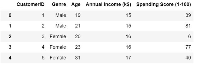

Top 5 rows of df df的前5行

The data set contains 5 features

数据集包含5个特征

问题陈述：我们需要根据人们的年收入(k $)和他们的花费(支出得分(1–100))对他们进行分组(Problem statement: we need to cluster the people basis on their Annual income (k$) and how much they Spend (Spending Score(1–100) ))

So our features for the clustering are Annual Income(k$) and Spending Score(1–100)

因此，我们的聚类功能是年收入(k $)和支出得分(1–100)

Spending score is nothing but a score gave the basis on how much they spend

支出分数不过是分数，是他们支出多少的依据

f1: Annual Income (k$)

f1：年收入(k $)

f2: Spending Score(1–100)

f2：支出得分(1-100)

Now we need to create an array with f1(x) and f2 (y) from data frame df

现在我们需要从数据帧df创建一个具有f1(x)和f2(y)的数组

# converting features f1 and f2 into an array 
X=df.iloc[:,[3,4]].values

We had features in array form now we can proceed to implement step

我们具有数组形式的功能，现在我们可以继续执行步骤

(iii)K-均值聚类：((iii) K-means Clustering :)

K-means Clustering is Centroid based algorithm

K-均值聚类是基于质心的算法

K = no .of clusters =Hyperparameter

K =簇数=超参数

We find K value using the Elbow method

我们用弯头法找到K值

K-means objective function is argmin (sum(||x-c||)²

K均值目标函数为argmin(sum(|| xc ||)²

where x = data point in the cluster

其中x =集群中的数据点

c= centroid of the cluster

c =群集的质心

objective: We need to minimize the square distance between the data point and centroid

目标：我们需要最小化数据点和质心之间的平方距离

If we have K-clusters then we have K-centroids

如果我们有K簇，那么我们就有K形心

Intracluster distance: Distances between data points in the same cluster

集群内距离：同一集群中数据点之间的距离

Intercluster distance: Distances between different clusters

集群间距离：不同集群之间的距离

Our main aim to choose the clusters which have small intracluster distance and large intercluster distance

我们的主要目标是选择集群内距离较小和集群间距离较大的集群

We use K-means++ initialization(probabilistic approach)

我们使用K-means ++初始化(概率方法)

from sklearn.cluster import KMeans# objective function is nothing but argmin of c (sum of (|x-c|)^2 )  c: centroid ,x=point in data setobjective_function=[] 
for i in range(1,11):
    clustering=KMeans(n_clusters=i, init='k-means++')
    clustering.fit(X)
    objective_function.append(clustering.inertia_)#inertia is calculaing min intra cluster distance
# objective function contains min intra cluster distances objective_function

objective_function : min intracluster distances

objective_function：群集内最小距离

[269981.28000000014,
 183116.4295463669,
 106348.37306211119,
 73679.78903948837,
 44448.45544793369,
 37233.81451071002,
 31599.13139461115,
 25012.917069885472,
 21850.16528258562,
 19701.35225128174]

We tried K value in the in-between 1 to 10, we don’t know which is best K surely

我们在1到10之间尝试了K值，但我们不确定K哪个最好

So to know best K we do Hyperparameter optimization

因此，要最了解K，我们需要进行超参数优化

Elbow method: Hyperparameter optimization

弯头法：超参数优化

# for finding optimal no of clusters we use elbow technique 
# Elbow technique is plot between no of clusters and objective_function 
# we take k at a point where the objective function value have elbow shape 
plt.plot(range(1,11),objective_function)
plt.title(‘The Elbow Method’)
plt.xlabel(‘Number of Clusters K’)
plt.ylabel(‘objective_function’)
plt.show()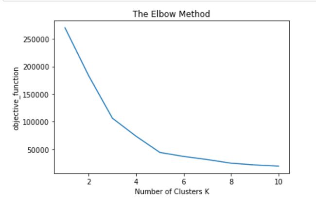

Hyperparameter optimization 超参数优化

In the above plot at K=5, we got elbow joint we consider optimum K=5

在以上K = 5的图中，我们得到了肘关节，我们认为最优K = 5

Now we train a model with an optimum K value

现在我们训练一个具有最佳K值的模型

# Training the model with optimal no of clusters

＃在没有最佳聚类的情况下训练模型

# Training the model with optimal no of clusterstuned_clustering=KMeans(n_clusters=5,init=’kmeans++’,random_state=0)
labels=tuned_clustering.fit_predict(X)# x and y  coordinates of all clusters
# Centroids of clusters
tuned_clustering.cluster_centers_[:]

labels return: predicted clusters

标签返回：预测簇

array([3, 1, 3, 1, 3, 1, 3, 1, 3, 1, 3, 1, 3, 1, 3, 1, 3, 1, 3, 1, 3, 1,
       3, 1, 3, 1, 3, 1, 3, 1, 3, 1, 3, 1, 3, 1, 3, 1, 3, 1, 3, 1, 3, 0,
       3, 1, 0, 0, 0, 0, 0, 0, 0, 0, 0, 0, 0, 0, 0, 0, 0, 0, 0, 0, 0, 0,
       0, 0, 0, 0, 0, 0, 0, 0, 0, 0, 0, 0, 0, 0, 0, 0, 0, 0, 0, 0, 0, 0,
       0, 0, 0, 0, 0, 0, 0, 0, 0, 0, 0, 0, 0, 0, 0, 0, 0, 0, 0, 0, 0, 0,
       0, 0, 0, 0, 0, 0, 0, 0, 0, 0, 0, 0, 0, 2, 4, 2, 0, 2, 4, 2, 4, 2,
       0, 2, 4, 2, 4, 2, 4, 2, 4, 2, 0, 2, 4, 2, 4, 2, 4, 2, 4, 2, 4, 2,
       4, 2, 4, 2, 4, 2, 4, 2, 4, 2, 4, 2, 4, 2, 4, 2, 4, 2, 4, 2, 4, 2,
       4, 2, 4, 2, 4, 2, 4, 2, 4, 2, 4, 2, 4, 2, 4, 2, 4, 2, 4, 2, 4, 2,
       4, 2])

tuned_clustering.cluster_centers_[:] return : centroid coordinates of each cluster

tuned_clustering.cluster_centers_ [：]返回：每个群集的质心坐标

array([[55.2962963 , 49.51851852],
       [25.72727273, 79.36363636],
       [86.53846154, 82.12820513],
       [26.30434783, 20.91304348],
       [88.2       , 17.11428571]])

Visualizing the clusters

可视化集群

# visualizing the clustersplt.scatter(X[labels==0,0],X[labels==0,1],c=’green’,label=’cluster1')
plt.scatter(X[labels==1,0],X[labels==1,1],c=’yellow’,label=’cluster2')
plt.scatter(X[labels==2,0],X[labels==2,1],c=’red’,label=’cluster3')
plt.scatter(X[labels==3,0],X[labels==3,1],c=’orange’,label=’cluster4')
plt.scatter(X[labels==4,0],X[labels==4,1],c=’blue’,label=’cluster5')plt.scatter(tuned_clustering.cluster_centers_[:,0],tuned_clustering.cluster_centers_[:,1],s=300,c=’black’,label=’centroid’)plt.title(‘Clusters of customers’)
plt.xlabel(‘Annual Income(K$)’)
plt.ylabel(‘Spending Score(1–100)’)
plt.legend()
plt.show()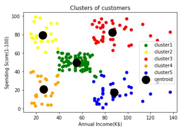

Clustering people Based on Annual Income and spending 根据年收入和支出对人进行聚类

Evaluation: How good our clustering is

评估：我们的集群有多好

To check how good our clustering we use the Silhouette coefficient

为了检查聚类的效果，我们使用Silhouette系数

Silhouette coefficient 轮廓系数

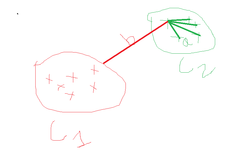
In the above diagram, we have two clusters C1 and C2

在上图中，我们有两个集群C1和C2

a= intracluster distance

a =集群内距离

b=intercluster distance

b =集群间距离

Silhouette coefficient= b-a/max(b,a)

轮廓系数= ba / max(b，a)

If our clustering is good then we have small intracluster distance then the Silhouette coefficient value is positive

如果聚类良好，则集群内距离较小，则Silhouette系数值为正

If our clustering is bad then we have large intracluster distance then the Silhouette coefficient value is negative

如果聚类不好，则集群内距离较大，则Silhouette系数值为负

Silhouette coefficient lies in between -1 and 1

轮廓系数在-1和1之间

If the value moves towards 1 then clustering is good

如果该值接近1，则说明聚类良好

If the value moves towards <0 then clustering is bad

如果该值趋于<0，则聚类不好

from sklearn import metrics
metrics.silhouette_score(X, tuned_clustering.labels_,
metric='euclidean')

We got the Silhouette coefficient value is 0.553931997444648

我们得到的Silhouette系数值为0.553931997444648

It’s moving towards 1 so our clustering is good

它正在接近1，所以我们的聚类很好

If you want to visualize the Silhouette coefficient

如果要可视化轮廓系数

# visualizing Silhouette coefficientfor n_clusters in range(2,10):
 # Create a subplot with 1 row and 2 columns
 fig, (ax1, ax2) = plt.subplots(1, 2)
 fig.set_size_inches(18, 7)# The 1st subplot is the silhouette plot
 # The silhouette coefficient can range from -1, 1 but in this example all
 # lie within [-0.1, 1]
 ax1.set_xlim([-0.1, 1])
 # The (n_clusters+1)*10 is for inserting blank space between silhouette
 # plots of individual clusters, to demarcate them clearly.
 ax1.set_ylim([0, len(X) + (n_clusters + 1) * 10])# Initialize the clusterer with n_clusters value and a random generator
 # seed of 10 for reproducibility.
 clusterer = KMeans(n_clusters=n_clusters, random_state=10)
 cluster_labels = clusterer.fit_predict(X)# The silhouette_score gives the average value for all the samples.
 # This gives a perspective into the density and separation of the formed
 # clusters
 silhouette_avg = silhouette_score(X, cluster_labels)
 print(“For n_clusters =”, n_clusters,
 “The average silhouette_score is :”, silhouette_avg)# Compute the silhouette scores for each sample
 sample_silhouette_values = silhouette_samples(X, cluster_labels)y_lower = 10
 for i in range(n_clusters):
 # Aggregate the silhouette scores for samples belonging to
 # cluster i, and sort them
 ith_cluster_silhouette_values = \
 sample_silhouette_values[cluster_labels == i]ith_cluster_silhouette_values.sort()size_cluster_i = ith_cluster_silhouette_values.shape[0]
 y_upper = y_lower + size_cluster_icolor = cm.nipy_spectral(float(i) / n_clusters)
 ax1.fill_betweenx(np.arange(y_lower, y_upper),
 0, ith_cluster_silhouette_values,
 facecolor=color, edgecolor=color, alpha=0.7)# Label the silhouette plots with their cluster numbers at the middle
 ax1.text(-0.05, y_lower + 0.5 * size_cluster_i, str(i))# Compute the new y_lower for next plot
 y_lower = y_upper + 10 # 10 for the 0 samplesax1.set_title(“The silhouette plot for the various clusters.”)
 ax1.set_xlabel(“The silhouette coefficient values”)
 ax1.set_ylabel(“Cluster label”)# The vertical line for average silhouette score of all the values
 ax1.axvline(x=silhouette_avg, color=”red”, linestyle=” — “)ax1.set_yticks([]) # Clear the yaxis labels / ticks
 ax1.set_xticks([-0.1, 0, 0.2, 0.4, 0.6, 0.8, 1])# 2nd Plot showing the actual clusters formed
 colors = cm.nipy_spectral(cluster_labels.astype(float) / n_clusters)
 ax2.scatter(X[:, 0], X[:, 1], marker=’.’, s=30, lw=0, alpha=0.7,
 c=colors, edgecolor=’k’)# Labeling the clusters
 centers = clusterer.cluster_centers_
 # Draw white circles at cluster centers
 ax2.scatter(centers[:, 0], centers[:, 1], marker=’o’,
 c=”white”, alpha=1, s=200, edgecolor=’k’)for i, c in enumerate(centers):
 ax2.scatter(c[0], c[1], marker=’$%d$’ % i, alpha=1,
 s=50, edgecolor=’k’)ax2.set_title(“The visualization of the clustered data.”)
 ax2.set_xlabel(“Feature space for the 1st feature”)
 ax2.set_ylabel(“Feature space for the 2nd feature”)plt.suptitle((“Silhouette analysis for KMeans clustering on sample data “
 “with n_clusters = %d” % n_clusters),
 fontsize=14, fontweight=’bold’)plt.show()

For n_clusters = 2 The average silhouette_score is : 0.3273163942500746For n_clusters = 3 The average silhouette_score is : 0.46761358158775435For n_clusters = 4 The average silhouette_score is : 0.4931963109249047For n_clusters = 5 The average silhouette_score is : 0.553931997444648For n_clusters = 6 The average silhouette_score is : 0.5379675585622219For n_clusters = 7 The average silhouette_score is : 0.5270287298101395For n_clusters = 8 The average silhouette_score is : 0.4548653400650936For n_clusters = 9 The average silhouette_score is : 0.4595491760122954

对于n_clusters = 2的平均silhouette_score为：0.3273163942500746对于n_clusters = 3的平均silhouette_score为：0.46761358158775435对于n_clusters = 4的平均silhouette_score为：0.4931963109249047对于n_clusters = 5的平均silhouette_score是：0.553931997444648对于n_clusters = 6的平均值为0.5：0.527331997444648对于n_clusters = 6对于n_clusters = 7，平均silhouette_score为：0.5270287298101395对于n_clusters = 8，平均silhouette_score为：0.4548653400650936对于n_clusters = 9，平均silhouette_score为：0.4595491760122954

K=5 Silhouette coefficient K = 5轮廓系数

If we observe the above scores for k=5 we have a high Silhouette coefficient

如果我们观察到k = 5的上述得分，我们的剪影系数就很高

If we observe the above plot no negative movements in clusters everything moving towards 1

如果我们观察上面的图，群集中没有负向运动，一切都朝着1移动

So we can conclude our clustering is good

所以我们可以得出结论，聚类是好的

(iv)层次聚类：((iv) Hierarchical Clustering :)

Hierarchical clustering is tree-based clustering

分层聚类是基于树的聚类

Dendrogram: It‘s a tree-like a diagram that records the sequence of merges

树状图：这是一个树状图，记录了合并的顺序

In Hierarchical clustering, we use Agglomerative clustering

在分层聚类中，我们使用聚集聚类

Step1: consider each data point as a cluster

步骤1：将每个数据点视为一个群集

Step2: merge clusters based on their similarity (distance)

步骤2：根据相似度(距离)合并聚类

if two clusters are very near to each other group those two clusters into one cluster

如果两个群集彼此非常靠近，则将这两个群集合并为一个群集

Repeat until only a single cluster remains

重复直到只剩下一个集群

In Agglomerative clustering no need to give no of clusters as hyperparameters we can stop hierarchy how many clusters we want

在聚集聚类中，不需要给出任何聚类作为超参数，我们可以停止层次结构，我们想要多少个聚类

So no.of clusters is not a hyperparameter

所以簇数不是一个超参数

# Dendogramimport scipy.cluster.hierarchy as schcluster_visualising=sch.dendrogram(sch.linkage(df.iloc[:,[3,4]].values,method=’ward’))
plt.title(‘Dendrogram’)
plt.xlabel(‘Customers’)
plt.ylabel(‘Euclidean distances’)
plt.show()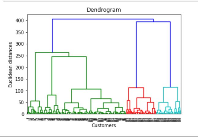

Dendrogram 树状图

If we observe the above dendrogram, it groups the customers according to min euclidean distance

如果我们观察上述树状图，它会根据最小欧几里德距离对客户进行分组

No.of clusters from dendrogram =We select the largest vertical line which can not cut by horizontal line

树状图的簇数=我们选择不能被水平线割断的最大垂直线

From the dendrogram, we choose K=5 =no of clusters

从树状图中，我们选择K = 5 =没有簇

For cluster similarity, we use the ward method

对于群集相似性，我们使用病房方法

Ward method less susceptible to noise and outliers

病房法不易受噪声和离群值的影响

# AgglomerativeClustering Model initializationfrom sklearn.cluster import AgglomerativeClusteringclustering_model=AgglomerativeClustering(n_clusters = 5, affinity = ‘euclidean’, linkage = ‘ward’)clustering_model.fit(df.iloc[:,[3,4]].values)# Predicting clusters
clustering_prediction=clustering_model.fit_predict(df.iloc[:,[3,4]])

clustering_predictoin return: Predicted clusters

clustering_predictoin返回：预测的集群

array([4, 3, 4, 3, 4, 3, 4, 3, 4, 3, 4, 3, 4, 3, 4, 3, 4, 3, 4, 3, 4, 3,
       4, 3, 4, 3, 4, 3, 4, 3, 4, 3, 4, 3, 4, 3, 4, 3, 4, 3, 4, 3, 4, 1,
       4, 1, 1, 1, 1, 1, 1, 1, 1, 1, 1, 1, 1, 1, 1, 1, 1, 1, 1, 1, 1, 1,
       1, 1, 1, 1, 1, 1, 1, 1, 1, 1, 1, 1, 1, 1, 1, 1, 1, 1, 1, 1, 1, 1,
       1, 1, 1, 1, 1, 1, 1, 1, 1, 1, 1, 1, 1, 1, 1, 1, 1, 1, 1, 1, 1, 1,
       1, 1, 1, 1, 1, 1, 1, 1, 1, 1, 1, 1, 1, 2, 1, 2, 1, 2, 0, 2, 0, 2,
       1, 2, 0, 2, 0, 2, 0, 2, 0, 2, 1, 2, 0, 2, 1, 2, 0, 2, 0, 2, 0, 2,
       0, 2, 0, 2, 0, 2, 1, 2, 0, 2, 0, 2, 0, 2, 0, 2, 0, 2, 0, 2, 0, 2,
       0, 2, 0, 2, 0, 2, 0, 2, 0, 2, 0, 2, 0, 2, 0, 2, 0, 2, 0, 2, 0, 2,
       0, 2], dtype=int64)

Visualizing clusters

可视化集群

plt.scatter(df.iloc[:,[3,4]].values[clustering_prediction == 0, 0], df.iloc[:,[3,4]].values[clustering_prediction == 0, 1], s = 100, c = ‘green’, label = ‘Cluster 1’)plt.scatter(df.iloc[:,[3,4]].values[clustering_prediction == 1, 0], df.iloc[:,[3,4]].values[clustering_prediction == 1, 1], s = 100, c = ‘red’, label = ‘Cluster 2’)plt.scatter(df.iloc[:,[3,4]].values[clustering_prediction == 2, 0], df.iloc[:,[3,4]].values[clustering_prediction == 2, 1], s = 100, c = ‘blue’, label = ‘Cluster 3’)plt.scatter(df.iloc[:,[3,4]].values[clustering_prediction == 3, 0], df.iloc[:,[3,4]].values[clustering_prediction == 3, 1], s = 100, c = ‘yellow’, label = ‘Cluster 4’)plt.scatter(df.iloc[:,[3,4]].values[clustering_prediction == 4, 0], df.iloc[:,[3,4]].values[clustering_prediction == 4, 1], s = 100, c = ‘orange’, label = ‘Cluster 5’)plt.title(‘Clusters of customers’)
plt.xlabel(‘Annual Income (k$)’)
plt.ylabel(‘Spending Score (1–100)’)
plt.legend()
plt.show()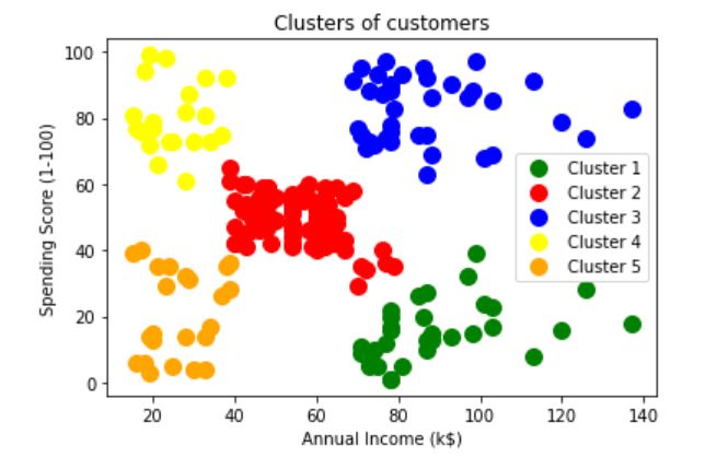

Clustering of people basis on their Annual Income and spending 根据人们的年收入和支出进行人群分组

Evaluation

评价

from sklearn import metrics
metrics.silhouette_score(df.iloc[:,[3,4]].values, clustering_prediction , metric='euclidean')

Silhouette coefficient: 0.5529945955148897

轮廓系数：0.5529945955148897

The coefficient moving towards 1 so clustering is good

系数接近1，所以聚类很好

(v)DBSCAN群集：((v) DBSCAN Clustering :)

DBSCAN is a density-based clustering

DBSCAN是基于密度的集群

We need to know the terms before implementing

在实施之前，我们需要了解术语

Dense region, Sparse region, Core point, Border point, Noise point , Density edge , Density connected points

密集区域，稀疏区域，核心点，边界点，噪声点，密度边缘，密度连接点

please refer the below link to understand the above-mentioned terms

请参考以下链接以了解上述条款

In DBSCAN Min points and epsilon are the hyperparameters

在DBSCAN中Min点和epsilon是超参数

Step1: For every point in the dataset we need to label data point belong to whether core point /border point/noise point

步骤1：对于数据集中的每个点，我们需要标记数据点是否属于核心点/边界点/噪声点

Step2: Remove all noise points

步骤2：移除所有杂讯点

Step3: For each core point ‘p’ which is not assigned to a cluster

步骤3：对于未分配给集群的每个核心点“ p”

we create a new cluster with not assigned core point and add all points that are density connected to not assigned core point into this new cluster

我们创建一个未分配核心点的新群集，并将所有密度连接到未分配核心点的点添加到此新群集中

Step4: each border point assign to the nearest core points cluster

步骤4：将每个边界点分配给最近的核心点群集

Hyperparameter optimization:

超参数优化：

In DBSCAN Min points and epsilon are the hyperparameters

在DBSCAN中Min点和epsilon是超参数

Min points :

最低积分：

rule of thumb ==> Min points ≥dimensionality +1

经验法则==>最小点≥维度+1

If the data set is noisier then we use Min Points are larger because it removes noisy points easily

如果数据集噪声较大，则我们使用的最小点数较大，因为它可以轻松消除噪声点

Epsilon (radius): Elbow method

Epsilon(半径)：肘部法

step1: for every data point (x) we compute distance (d)

步骤1：对于每个数据点(x)，我们计算距离(d)

stpe2: sort distances in increasing order

stpe2：按递增顺序排列距离

then plot the graph between distance and point index

然后在距离和点索引之间绘制图形

We choose the optimum distance(epsilon) d, where the sharp rise in the graph

我们选择最佳距离ε，曲线图中的急剧上升

# we use nearestneighbors for calculating distance between pointsfrom sklearn.neighbors import NearestNeighbors
# calculating distancesneigh=NearestNeighbors(n_neighbors=2)
distance=neigh.fit(X)
# indices and distance values
distances,indices=distance.kneighbors(X)
# Now sorting the distance increasing ordersorting_distances=np.sort(distances,axis=0)
# sorted distancessorted_distances=sort_distances[:,1]# plot between distance vs epsilonplt.plot(sorted_distances)
plt.xlabel(‘Distance’)
plt.ylabel(‘Epsilon’)
plt.show()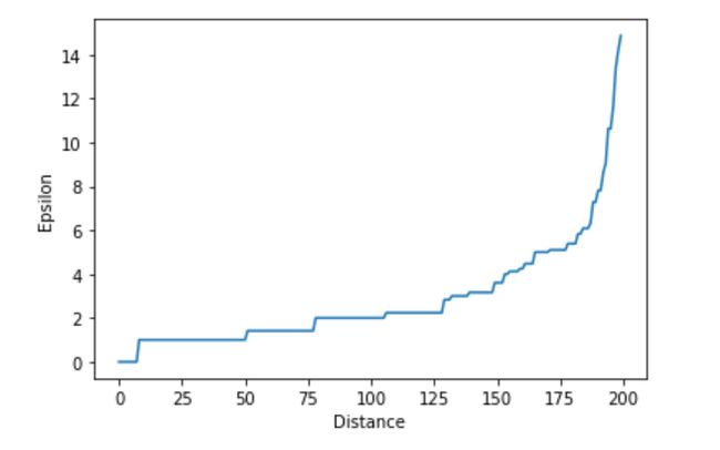

Epsilon optimization Epsilon优化

If we observe the graph, at epsilon is equal to 9 sharp rises in the graph so we choose epsilon(radius) as 9

如果我们观察该图，则epsilon等于图中的9个急剧上升，因此我们选择epsilon(radius)为9

Implementing DBSCAN with optimized hyperparameters

使用优化的超参数实现DBSCAN

from sklearn.cluster import DBSCAN# intializing DBSCANclustering_model=DBSCAN(eps=9,min_samples=4)# fit the model to Xclustering_model.fit(X)# predicted labels by DBSCANpredicted_labels=clustering_model.labels_
# visualzing clustersplt.scatter(X[:,0], X[:,1],c=predicted_labels, cmap='Paired')
plt.xlabel('Annual Income')
plt.ylabel('Spending Score')
plt.title("DBSCAN")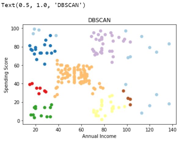

Evaluation :

评价：

from sklearn import metricsmetrics.silhouette_score(X, predicted_labels)

Silhouette coefficient: 0.4259680122384905

轮廓系数：0.4259680122384905

Silhouette coefficient moving towards 1 so our clustering is good

轮廓系数接近1，因此我们的聚类良好

(vi)结论：((vi) Conclusion :)

I hope you find this article is helpful , Please give me your feedback that will helpful for me

希望本文对您有所帮助，请给我您的反馈意见，以对我有所帮助

(vii)参考资料：((vii) References :)

翻译自: https://medium.com/analytics-vidhya/practical-implementation-of-k-means-hierarchical-and-dbscan-clustering-on-dataset-with-bd7f3d13ef7f

dbscan聚类高维数据