Factorization Machines. VS Support Vector Machines.(理解+实现)
FM是什么?
FM(Factorization Machine,因子分解机)主要是为了解决数据稀疏的情况下,特征怎样组合的问题。

为什么使用FM?
正如FM是什么说的,FM主要用来解决:1.数据稀疏 2.特征组合。
1.数据稀疏:现如今在推荐系统中存在这种问题,例如一个书店网上商城,商城中有几百万本书籍,大部分用户最多也就买几本或者几十本,在一条用户向量中绝大部分的值都是0。
2.特征组合:在现在的机器学习建模中,如果直接对特征进行建模,会使我们忽略了特征与特征之间的交互关系(比如男生喜欢运动类,女生喜欢衣服类等),这些交互关系往往十分重要。这就需要我们建立特征与特征之间的交互关系,从而提高模型的效果。
FM算法就可以解决以上两个问题:
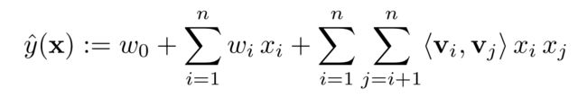
引入了交叉项特征解决特征组合:
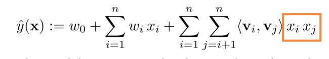
引入了隐变量解决数据稀疏:
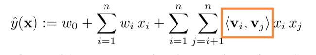
这里特别说明一下:
不是不用Wij,而是Wij不容易得出。使用Wij在训练数据的时候,如果可以把Wij训练出来,就必须Xi和Xj同时不为0,如果有一个为0了,那么Wij就无法得到,尤其使对于稀疏数据就更无法得到。所以引入了隐变量Vi和Vj去代替Wij,不用满足Xi和Xj同时不为0。这样Vi和Vj可以单独被训练出来。

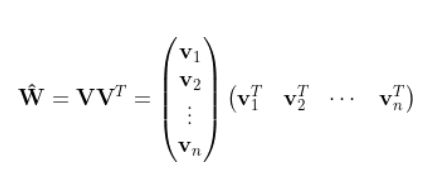
V是一个n * k维的,n是X的特征数,k是我们分解隐变量的维数(可以自己确定)。
则W = V * V .T or V.T * V (这里我感觉是矩阵分解,将Wij分解成两个相同的vector进行训练)
FM如何求解?
这个yhat的时间复杂度是O(K * N * N),我们可以把它优化成O(K * N )。实现了一个效果的提升。

《Factorization Machines》论文中说了可以处理三类问题:回归问题、二分类问题、和排序问题(我还没有遇到过,遇到后补)。
我们然后进行优化:先定义loss,再对yhat中的参数进行求导计算梯度。如下图所示。

 的计算见下图。

FM好处(Baseline SVM)?
1.在稀疏数据中,FM效果优于SVM。
2.FM可以直接在目标函数中学习,非线性的SVM学习需要用到对偶。
3.FM的模型式子与训练集无关,SVM的预测需要依赖于部分训练数据(支持向量)。
比较FM和SVM在二分类的效果:
代码实现:
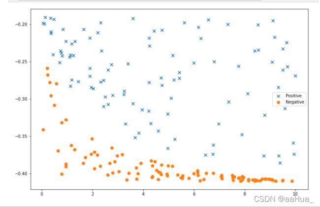
dataset:200条数据,前两列特征值,最后一列目标值。数据贴在最后。

数据图
FM模型(初学FM,手动实现FM,加深印象):
import numpy as np
import matplotlib.pyplot as plt
#导入数据集
def load_data(filename):
    data = open(filename)
    feature = []
    label = []
    for line in data.readlines():
        feature_tmp = []
        lines = line.strip().split("\t")
        for x in range(len(lines)-1):
            feature_tmp.append(float(lines[x]))
        label.append(int(lines[-1])* 2 -1)
        feature.append(feature_tmp)
    data.close()
    return feature ,label
#初始化参数值
def initialize_w_v(n, k):
    w = np.ones((n, 1))
    v = np.mat(np.zeros((n, k)))
    for i in range(n):
        for j in range(k):
            v[i, j] = np.random.normal(0,0.2)
    return w, v
#sigmoid函数
def sigmoid(x):
    return (1 / (1 + np.exp(-x)))
#得到损失值
def get_loss(predict, classlabels):
    m = np.shape(predict)[0]
    Loss = []
    error = 0
    for i in range(m):
        error -= np.log(sigmoid(predict[i] * classlabels[i]))
        Loss.append(error)
    return Loss
#预测output值函数
def prediction(dataMatrix ,w0, w, v):
    m = np.shape(dataMatrix)[0]
    result = []
    for x in range(m):
        inter_1 = dataMatrix[x] * v
        inter_2 = np.multiply(dataMatrix[x],dataMatrix[x]) * np.multiply(v, v)
        interaction  = 0.5 * np.sum(np.multiply(inter_1,inter_1) - inter_2)
        p = w0 + dataMatrix[x] * w + interaction
        pre = sigmoid(p[0, 0])
        result.append(pre)
    return result
#获得失误率
def getaccuracy(predict,classLabels):
    m = np.shape(predict)[0]
    allItem = 0
    error = 0
    for i in range(m):
        allItem += 1
        if float(predict[i])< 0.5 and classLabels[i] == 1.0:
            error += 1
        elif float(predict[i])>=0.5 and classLabels[i] == -1.0:
            error += 1
        else:
            continue
    return float(error)/allItem
#梯度下降
def SGD(dataMatrix, classLabels, k, max_iter, alpha):
    m ,n = np.shape(dataMatrix)
    acc = []
    gloss = []
    w0 = 0
    w,v = initialize_w_v(n,k)#初始化参数
    for it in range(max_iter):
        for x in range(m):
            v_1 = dataMatrix[x] * v
            v_2 = np.multiply(dataMatrix[x] ,dataMatrix[x]) * np.multiply(v,v)
            interaction = 0.5 * np.sum( np.multiply(v_1,v_1) - v_2)
            p = w0 + dataMatrix[x] * w + interaction
            q = sigmoid(classLabels[x] * p[0, 0])-1

            w0 = w0 - alpha * q * classLabels[x]
            for i in range(n):
                if dataMatrix[x, i] != 0:
                    w[i, 0] = w[i, 0] - alpha * q * classLabels[x] * dataMatrix[x, i]
                    for j in range(k):
                        v[i, j] = v[i, j] - alpha * q * classLabels[x] * (dataMatrix[x, i] * v_1[0, j]  - v[i, j] * dataMatrix[x, i] * dataMatrix[x, i])

        if it%250 == 0:
            print("\n迭代次数:" + str(it) + ",loss误差:" + str(get_loss(prediction(np.mat(dataMatrix), w0, w, v), classLabels)[-1])+ "  ,acc:" + str((1 -getaccuracy(prediction(np.mat(dataMatrix), w0, w, v),label))* 100))
            acc.append((1 - getaccuracy(prediction(np.mat(dataMatrix), w0, w, v),classLabels))* 100 )
            gloss.append(get_loss(prediction(np.mat(dataMatrix), w0, w, v), classLabels)[-1])
    return w0, w, v , acc, gloss
#获取数据
feature,label = load_data('train_data.txt')
#训练
w0, w, v , acc, gloss=SGD(np.mat(feature), label, k = 2, max_iter = 10000, alpha = 0.01)
#预测结果
predict_result = prediction(np.mat(feature), w0 ,w, v)
#准确率
1 - getaccuracy(predict_result ,label)
#画图
plt.clf()
plt.plot(range(0,10000,250),acc ,label='acc')
plt.plot(range(0,10000,250),gloss,label='loss')
plt.title("acc and loss ")
plt.xlabel('Number of Epochs')
plt.ylabel('acc or loss')
plt.legend()
plt.grid()
plt.show()
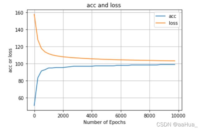

FM在本数据集上表现为99%
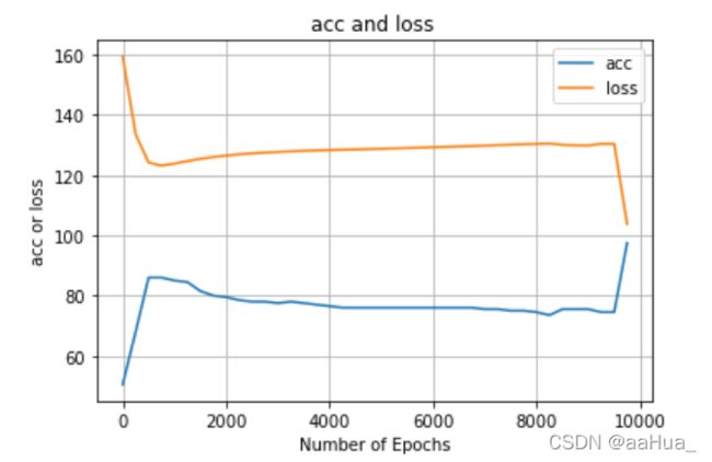
(lr不要调太大,否则图会出现这种情况,如下图)
SVM模型:
import numpy as np
import pandas as pd
import matplotlib.pyplot as plt
import seaborn as sb
from sklearn import svm
#导入数据集
def load_data(filename):
    data = open(filename)
    feature = []
    label = []
    for line in data.readlines():
        feature_tmp = []
        lines = line.strip().split("\t")
        for x in range(len(lines)-1):
            feature_tmp.append(float(lines[x]))
        label.append(int(lines[-1])* 2 -1)
        feature.append(feature_tmp)
    data.close()
    return feature ,label
#加载数据
feature ,label = load_data("train_data.txt")
#调用sklearn中的svm
svc = svm.SVC(C=100, gamma=10, probability=True,degree=2,kernel='poly')
#训练
svc.fit(feature, label)
#得分
svc.score(feature, label)
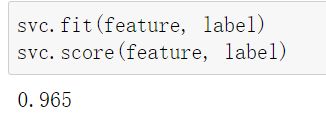
对比:
FM:99%
SVM:96.5%
数据:
8.42383194320181	-0.408530918340288	0
9.23508197146775	-0.409948204795973	0
0.580765279496576	-0.279597802215932	0
7.09767621267017	-0.406498441260137	0
4.67937536514234	-0.398978513749255	0
0.943442483964607	-0.390353722860601	0
3.74734509186577	-0.406970631021985	0
8.39393102401964	-0.408098172982057	0
0.959332381553160	-0.327607520319716	0
0.232976645546809	-0.267919464760288	0
8.80446107146714	-0.407059057326573	0
8.59938392690125	-0.409463220043359	0
8.95457694589616	-0.407156922375112	0
7.96098805532834	-0.404925626334067	0
0.323054757630367	-0.277907453214403	0
5.48175722168676	-0.405673387149798	0
7.79512012715714	-0.405554237820353	0
7.08253377287152	-0.403444252353187	0
6.16060448107641	-0.402178642303065	0
2.19119512788717	-0.374994207835389	0
6.39367188624695	-0.407775618172926	0
7.08725937669242	-0.401984304924651	0
5.79904363518889	-0.406311564806981	0
7.59045186538154	-0.404279834086207	0
3.43767463555210	-0.399625151711070	0
2.87283978693540	-0.383673362704480	0
8.39831970761900	-0.409923888575123	0
6.14553209617717	-0.398027016959763	0
0.640956937606998	-0.369389256091614	0
2.29934679549623	-0.390199749245145	0
8.44224693484357	-0.408805330232292	0
8.99502222039451	-0.407918113927482	0
8.83624008312127	-0.406908558560670	0
4.92895815278608	-0.400438153125454	0
9.48949088303997	-0.409507907710384	0
4.72531083707912	-0.388488084816166	0
2.79710704451344	-0.398760341218867	0
7.50798039275919	-0.402176743887395	0
8.48456070568963	-0.409573472614389	0
6.76039013462219	-0.399155829461459	0
4.95419059477074	-0.402920870029448	0
0.368705560882775	-0.295255777879522	0
3.16444939510907	-0.374571618600867	0
4.59626051785997	-0.407894572189662	0
0.490153434008910	-0.308314164887461	0
8.15134490163779	-0.409410678288747	0
7.90275758229961	-0.403723870611547	0
0.792283779528635	-0.400626399527537	0
5.14139837739626	-0.389768236579979	0
7.90627365243289	-0.408257660707080	0
0.953997866754101	-0.387163744616786	0
7.07159301485602	-0.403993824841355	0
9.06135640037553	-0.407768984132258	0
4.60341758246115	-0.397916532966483	0
6.14049890866498	-0.396185699910743	0
0.215329214059079	-0.258898195179039	0
5.55299812527370	-0.402812693630881	0
7.84043390068847	-0.409698820787648	0
1.94315237951002	-0.373588761269258	0
9.11121088568475	-0.408592842513344	0
2.98012686704141	-0.376214571346192	0
8.31904174333194	-0.408494949263143	0
0.0617846529338062	-0.340868672885575	0
8.15012626726182	-0.408131221643975	0
3.34934836292938	-0.408375749162869	0
5.35346540043212	-0.401516989385279	0
1.15862753436787	-0.362051199835335	0
8.14973224773878	-0.407970422188632	0
1.30092154826364	-0.367497518923388	0
9.51082762250197	-0.408822030204151	0
4.36731432815911	-0.403937404065732	0
1.63639911741812	-0.386052118856741	0
4.34680455530927	-0.404963242319624	0
5.54411463581684	-0.406131856090851	0
2.67898058380966	-0.386029299057639	0
6.49212676676911	-0.399635959788227	0
1.98095766638061	-0.353260659977698	0
9.85857911401332	-0.409731715702965	0
3.72624721185135	-0.391894215651133	0
3.04418081530650	-0.397177782029156	0
4.70877424186155	-0.400804752644355	0
2.08279213037150	-0.370806730680289	0
1.71073454775069	-0.378354524558988	0
2.76764193110911	-0.365288535360287	0
2.60636248760882	-0.401476620424844	0
7.52960877987452	-0.404993039099243	0
5.99643601412483	-0.399874324624253	0
4.36479759540816	-0.389384922905883	0
4.32073210555306	-0.382780916980243	0
0.787285208315720	-0.331534381633025	0
2.08438543917472	-0.393467876583496	0
4.98213558688768	-0.389168459685345	0
3.90159130065528	-0.385771872682800	0
7.55175246633567	-0.409057725558823	0
8.68762117721727	-0.407081041092895	0
4.45476757159167	-0.383674139566138	0
7.76549896072094	-0.405838601725101	0
6.23329124826219	-0.409628510931385	0
3.79021180613286	-0.399693570093771	0
4.52309238928843	-0.395367919485949	0
2.43758468710462	-0.309939998418769	1
6.44418448019331	-0.374723936417501	1
0.108671481485529	-0.199476534945679	1
3.23472132602922	-0.293911269333190	1
2.44178385018835	-0.275101689318301	1
0.481016991996002	-0.192982794728889	1
0.370857692202135	-0.211953271451565	1
5.23724591999750	-0.354020696656430	1
2.31740055767812	-0.277176863084907	1
4.24719365238813	-0.228720604973186	1
8.52967025477565	-0.200621670458921	1
1.18233156697587	-0.274076903571856	1
1.09122823571812	-0.243999645215050	1
2.02173302580917	-0.285987222107165	1
3.40157958868141	-0.252717387598389	1
6.56671655335725	-0.193815695710377	1
4.23709249848205	-0.218142740805575	1
1.89470124377699	-0.269331811708736	1
5.62107145721497	-0.197866145768924	1
0.442181978566363	-0.240539910325545	1
9.08335733334861	-0.250443920103596	1
8.54289949149346	-0.234576108061670	1
9.58048914374455	-0.312797618264376	1
4.21071321246505	-0.316157102407788	1
4.97486886565608	-0.365878657382866	1
8.78768695109643	-0.321746252520346	1
1.94010035906808	-0.284504821876978	1
9.50071876810555	-0.261254625802206	1
2.79092290897387	-0.294736667059161	1
4.42835500663540	-0.208733341730909	1
3.25337111859363	-0.289340840488577	1
7.75480499711548	-0.256121320230722	1
0.0601067147854828	-0.198420599896546	1
2.49753304116731	-0.297363143424683	1
1.12461072377156	-0.240865075131135	1
4.71228257009732	-0.271363789011752	1
9.34252613513342	-0.375946031143510	1
0.843081122373650	-0.206798239427842	1
5.09326655603538	-0.298924436083304	1
1.18717487407077	-0.225764713465440	1
2.60896221021649	-0.260828875403664	1
0.340567170451632	-0.191643171111526	1
9.32339305356395	-0.284591245201535	1
6.27445499304504	-0.218749932355235	1
8.75443656218165	-0.375860128116557	1
0.712694646768266	-0.251211368306295	1
5.41638852433666	-0.272060884009967	1
2.61870887856769	-0.306927321245432	1
7.36200224757743	-0.303688359058616	1
5.15489836245557	-0.241798486731131	1
9.91470220969572	-0.358627726808887	1
4.74387896326763	-0.281474800994315	1
4.23914505530651	-0.277643748743069	1
9.94279588232450	-0.373595713542861	1
0.138071308907622	-0.190271171365226	1
9.50180527233723	-0.232862772106994	1
0.742582446482145	-0.235530788445218	1
3.59237014923007	-0.192175481878045	1
9.39045198333577	-0.385328069458975	1
4.73261365346132	-0.207880132356065	1
1.43665183723223	-0.276445932905554	1
1.31465794513618	-0.222524617911456	1
3.30046965707428	-0.333016613374630	1
2.21316635113260	-0.210812844878435	1
7.88116832470351	-0.347570517509302	1
3.94844968752540	-0.314266793088863	1
5.98768064837655	-0.251301389475543	1
0.764400320140725	-0.238386704654004	1
2.31562057548408	-0.197609507341517	1
3.59415897605416	-0.306009583621716	1
0.959444038741402	-0.222606385961562	1
4.96117878536822	-0.320184560589757	1
7.32869253873543	-0.199698227443838	1
9.65718624060435	-0.224157687761801	1
1.89880655369980	-0.218112784562061	1
4.59724528984552	-0.342520285993113	1
3.83115222907876	-0.345264503383366	1
9.10505674005844	-0.194858902510535	1
6.98077467036255	-0.333072899621645	1
6.75437899881917	-0.361705241427897	1
9.68358853481333	-0.256771347021000	1
1.13187673107476	-0.282679813491173	1
0.358556369186400	-0.209628835794929	1
8.39618590956441	-0.235250064272360	1
9.99619620484049	-0.268975031963082	1
3.67237049360799	-0.351774945120537	1
2.35445411876548	-0.235625809877974	1
4.29008640794217	-0.332959541281784	1
5.42742747484534	-0.264438465444690	1
8.11606658953466	-0.292581532775660	1
9.18469883425862	-0.217003179402255	1
5.21837068366336	-0.274530530316992	1
6.79585182614347	-0.250119897154528	1
1.89061726771386	-0.258709988718971	1
6.16955623109348	-0.203747812388698	1
1.66149183322044	-0.206700226963393	1
2.74262556141998	-0.254027266166219	1
1.24804345641085	-0.241408809531456	1
0.808431917613837	-0.242017996831424	1
6.74094601972670	-0.373633464603415	1