在本教程中,我们将学习使用Seurat3对scATAC-seq和scRNA-seq的数据进行整合分析,使用一种新的数据转移映射方法,将scATAC-seq的数据基于scRNA-seq数据聚类的结果进行细胞分群,并进行整合分析。
对于scATAC-seq,我们还开发了一个独立的Signac包,可以用于单细胞ATAC-seq的数据分析及其整合分析,详细的使用方法可以参考Signac包官网的说明文档。
本示例中,我们将使用10X genomics测序平台产生的PBMC数据集(包含大约10K个细胞的scRNA-seq和scATAC-seq的测序数据)进行分析演示,整体的分析流程主要包括以下几个步骤:
- Estimate RNA-seq levels from ATAC-seq (quantify gene expression ‘activity’ from ATAC-seq reads)
- Learn the internal structure of the ATAC-seq data on its own (accomplished using LSI)
- Identify ‘anchors’ between the ATAC-seq and RNA-seq datasets
- Transfer data between datasets (either transfer labels for classification, or impute RNA levels in the ATAC-seq data to enable co-embedding)
基因表达活性的定量
首先,我们加载scATAC-seq数据产生的一个peak matrix,并将其整合合并成一个gene activity matrix。我们基于这样一个简单的假设:基因的表达活性可以简单的通过基因上下游2kb范围内覆盖的reads数的加和进行定量,最后获得一个gene x cell的表达矩阵。
# 加载所需的R包
library(Seurat)
library(ggplot2)
library(patchwork)
# 加载peak矩阵文件
peaks <- Read10X_h5("../data/atac_v1_pbmc_10k_filtered_peak_bc_matrix.h5")

# create a gene activity matrix from the peak matrix and GTF, using chromosomes 1:22, X, and Y.
# Peaks that fall within gene bodies, or 2kb upstream of a gene, are considered
# 使用CreateGeneActivityMatrix函数构建基因表达活性矩阵
activity.matrix <- CreateGeneActivityMatrix(peak.matrix = peaks, annotation.file = "../data/Homo_sapiens.GRCh37.82.gtf", seq.levels = c(1:22, "X", "Y"), upstream = 2000, verbose = TRUE)
构建Seurat对象
接下来,我们创建一个seurat对象存储scATAC-seq的数据,其中原始的peak counts存储在"ATAC"这个Assay中,基因表达活性的矩阵存储在"RNA"这个Assay中。对于原始的count,我们将进行QC过滤掉那些总counts数低于5k的细胞。
# 创建seurat对象
pbmc.atac <- CreateSeuratObject(counts = peaks, assay = "ATAC", project = "10x_ATAC")
pbmc.atac[["ACTIVITY"]] <- CreateAssayObject(counts = activity.matrix)
# meta信息
meta <- read.table("../data/atac_v1_pbmc_10k_singlecell.csv", sep = ",", header = TRUE, row.names = 1, stringsAsFactors = FALSE)
meta <- meta[colnames(pbmc.atac), ]
pbmc.atac <- AddMetaData(pbmc.atac, metadata = meta)
# 数据过滤
pbmc.atac <- subset(pbmc.atac, subset = nCount_ATAC > 5000)
pbmc.atac$tech <- "atac"
数据预处理
# 对基因表达活性矩阵进行标准化
DefaultAssay(pbmc.atac) <- "ACTIVITY"
pbmc.atac <- FindVariableFeatures(pbmc.atac)
pbmc.atac <- NormalizeData(pbmc.atac)
pbmc.atac <- ScaleData(pbmc.atac)
Here we perform latent semantic indexing to reduce the dimensionality of the scATAC-seq data. This procedure learns an ‘internal’ structure for the scRNA-seq data, and is important when determining the appropriate weights for the anchors when transferring information. We utilize Latent Semantic Indexing (LSI) to learn the structure of ATAC-seq data, as proposed in Cusanovich et al, Science 2015 and implemented in the RunLSI function. LSI is implemented here by performing computing the term frequency-inverse document frequency (TF-IDF) followed by SVD.
# 对原始的peak矩阵进行降维处理
DefaultAssay(pbmc.atac) <- "ATAC"
VariableFeatures(pbmc.atac) <- names(which(Matrix::rowSums(pbmc.atac) > 100))
# 使用LSI方法进行降维
pbmc.atac <- RunLSI(pbmc.atac, n = 50, scale.max = NULL)
pbmc.atac <- RunUMAP(pbmc.atac, reduction = "lsi", dims = 1:50)
# 加载scRNA-seq数据
pbmc.rna <- readRDS("../data/pbmc_10k_v3.rds")
pbmc.rna$tech <- "rna"
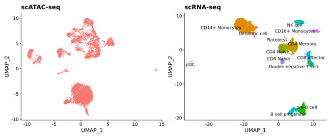
# 数据可视化
p1 <- DimPlot(pbmc.atac, reduction = "umap") + NoLegend() + ggtitle("scATAC-seq")
p2 <- DimPlot(pbmc.rna, group.by = "celltype", label = TRUE, repel = TRUE) + NoLegend() + ggtitle("scRNA-seq")
p1 + p2
接下来,我们将对scATAC-seq和scRNA-seq的数据进行整合分析。
# 识别整合的anchors,使用scRNA-seq的数据作为参照
transfer.anchors <- FindTransferAnchors(reference = pbmc.rna, query = pbmc.atac, features = VariableFeatures(object = pbmc.rna), reference.assay = "RNA", query.assay = "ACTIVITY", reduction = "cca")
# 使用TransferData函数进行数据转移映射
celltype.predictions <- TransferData(anchorset = transfer.anchors, refdata = pbmc.rna$celltype, weight.reduction = pbmc.atac[["lsi"]])
# 添加预测信息
pbmc.atac <- AddMetaData(pbmc.atac, metadata = celltype.predictions)
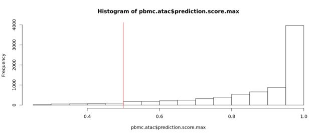
然后,我们可以检查预测分数的分布,并可以选择过滤掉那些得分较低的细胞。在这里,我们发现超过95%的细胞得分为0.5或更高。
hist(pbmc.atac$prediction.score.max)
abline(v = 0.5, col = "red")
table(pbmc.atac$prediction.score.max > 0.5)
##
## FALSE  TRUE
##   290  7576
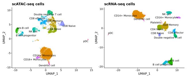
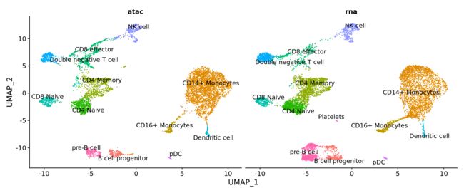
同样的,我们可以通过UMAP降维可视化scATAC-seq数据预测的细胞类型,并发现所转移的标签与scRNA-seq数据UMAP结果的结构高度一致。
# 数据过滤
pbmc.atac.filtered <- subset(pbmc.atac, subset = prediction.score.max > 0.5)
pbmc.atac.filtered$predicted.id <- factor(pbmc.atac.filtered$predicted.id, levels = levels(pbmc.rna))  # to make the colors match
# 数据可视化
p1 <- DimPlot(pbmc.atac.filtered, group.by = "predicted.id", label = TRUE, repel = TRUE) + ggtitle("scATAC-seq cells") + NoLegend() + scale_colour_hue(drop = FALSE)
p2 <- DimPlot(pbmc.rna, group.by = "celltype", label = TRUE, repel = TRUE) + ggtitle("scRNA-seq cells") + NoLegend()
p1 + p2
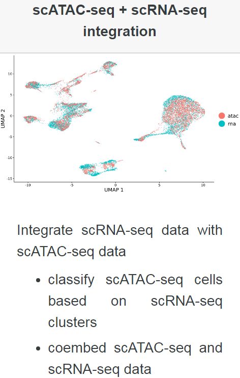
共嵌入联合可视化分析
最后,为了将所有的细胞一起可视化,我们可以将scRNA-seq和scATAC-seq细胞共同嵌入到同一低维空间中。在这里,我们首先使用先前识别出的相同anchors来转移映射细胞类型标签,以估算填充scATAC-seq细胞的RNA-seq值。然后,我们合并测得的和估算填充的scRNA-seq数据,并运行标准UMAP进行降维可视化所有的细胞。请注意,此步骤仅用于可视化目的,不是数据转移映射分析的必要部分。
# note that we restrict the imputation to variable genes from scRNA-seq, but could impute the full transcriptome if we wanted to
genes.use <- VariableFeatures(pbmc.rna)
refdata <- GetAssayData(pbmc.rna, assay = "RNA", slot = "data")[genes.use, ]

# refdata (input) contains a scRNA-seq expression matrix for the scRNA-seq cells.  imputation (output) will contain an imputed scRNA-seq matrix for each of the ATAC cells
imputation <- TransferData(anchorset = transfer.anchors, refdata = refdata, weight.reduction = pbmc.atac[["lsi"]])

# this line adds the imputed data matrix to the pbmc.atac object
pbmc.atac[["RNA"]] <- imputation
# 进行merge合并
coembed <- merge(x = pbmc.rna, y = pbmc.atac)

# Finally, we run PCA and UMAP on this combined object, to visualize the co-embedding of both datasets
coembed <- ScaleData(coembed, features = genes.use, do.scale = FALSE)
coembed <- RunPCA(coembed, features = genes.use, verbose = FALSE)
coembed <- RunUMAP(coembed, dims = 1:30)
coembed$celltype <- ifelse(!is.na(coembed$celltype), coembed$celltype, coembed$predicted.id)
Here we plot all cells colored by either their assigned cell type (from the 10K dataset) or their predicted cell type from the data transfer procedure.
p1 <- DimPlot(coembed, group.by = "tech")
p2 <- DimPlot(coembed, group.by = "celltype", label = TRUE, repel = TRUE)
p1 + p2

How can I further investigate unmatched groups of cells that only appear in one assay?
在查看UMAP嵌和数据可视化的结果中,我们发现有几种细胞似乎仅在一种测序类型数据中存在。例如,血小板细胞仅出现在scRNA-seq数据中。这些细胞被认为正在经历从巨核细胞到血小板细胞分化的过程中,因此要么完全缺乏核物质,要么它们的染色质状态与其转录的过程不一致。因此,我们不能期望它们在此分析中会保持一致。
DimPlot(coembed, split.by = "tech", group.by = "celltype", label = TRUE, repel = TRUE) + NoLegend()
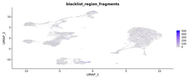
此外,我们还发现在B细胞祖细胞旁边似乎也有一个细胞类群,该类群只存在于scATAC-seq数据中,并且与scRNA-seq数据的细胞整合得不好。对这些细胞的元数据信息进一步检查发现,大量的reads映射到black list区域(由10x Genomics QC指标提供)。这表明这些细胞可能代表了死亡或垂死的细胞,环境中的DNA或其他人工的污染,导致其不存在于scRNA-seq数据集中。
coembed$blacklist_region_fragments[is.na(coembed$blacklist_region_fragments)] <- 0
FeaturePlot(coembed, features = "blacklist_region_fragments", max.cutoff = 500)
How can I evaluate the success of cross-modality integration?
- Overall, the prediction scores are high which suggest a high degree of confidence in our cell type assignments.
- We observe good agreement between the scATAC-seq only dimensional reduction (UMAP plot above) and the transferred labels.
- The co-embedding based on the same set of anchors gives good mixing between the two modalities.
- When we collapse the ATAC-seq reads on a per-cluster basis into “pseudo bulk” profiles, we observe good concordance with the chromatin patterns observed in bulk data
参考来源:https://satijalab.org/seurat/v3.1/atacseq_integration_vignette.html