使用Seaborn和Matplotlib进行数据可视化简介

We live in an online era, we create 2.5 quintillion bytes of data each day. By the time you are reading this article, the number has increased already! That is a huge, really huge. Data visualization is the tool to harness its power. In the world of data science, one of the widely used libraries in python for the same is seaborn — an easy-to-use yet powerful tool.

我们生活在一个在线时代，我们每天创建2.5兆字节的数据。 在您阅读本文时，数量已经增加了！ 那是巨大的，非常巨大的。 数据可视化是利用其功能的工具。 在数据科学领域，python中广泛使用的同一个库之一就是seaborn －一种易于使用但功能强大的工具。

Seaborn is an advanced data visualization library built on top of the matplotlib library — a plotting library for the Python programming language and its numerical mathematics extension NumPy. For this tutorial, you need a jupyter notebook/google colab or any other such .ipynb supporting the application. Without further due, let’s get started by importing all the necessary libraries.

Seaborn是在matplotlib库之上构建的高级数据可视化库，该库是Python编程语言及其数字数学扩展NumPy的绘图库。 对于本教程，您需要一个jupyter笔记本/ google colab或任何其他支持该应用程序的.ipynb。 无需进一步说明，让我们开始导入所有必需的库。

搭建环境 (Setting up the environment)

Run the following code in your notebook to import pandas, matplotlib, and seaborn libraries.

[R未在您的笔记本进口大熊猫，matplotlib和seaborn库下面的代码。

import pandas as pd
import matplotlib.pyplot as plt
%matplotlib inline
import seaborn as sns

If you do not have these libraries already installed, then use the following command to install them from your jupyter notebook and then use the above command to import them.

如果尚未安装这些库，请使用以下命令从jupyter笔记本中安装它们，然后使用上述命令导入它们。

!pip install pandas
!pip install matplotlib
!pip install seaborn

导入和理解数据(Importing and understanding data)

We will be using the pokemon dataset for this exercise, you can get it from here or just run the following code

我们将在此练习中使用pokemon数据集，您可以从此处获取它，也可以运行以下代码

file_path = "https://raw.githubusercontent.com/sanketkangle/Exploratory-Data-Analysis/master/Seaborn_tutorial/Pokemon.csv"
df = pd.read_csv(file_path, index_col = 0)
df.head()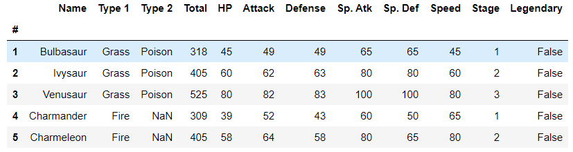

You should be able to see this combat stats data for the original 151 Pokémon.

您应该能够看到原始151神奇宝贝的战斗状态数据。

使用Seaborn的线图 (Line plot using Seaborn)

In the line chart, the measurement points are ordered (typically by their x-axis value) and joined with straight line segments. A line chart is often used to visualize a trend in data over intervals of time — a time series — thus the line is often drawn chronologically. In these cases, they are known as run charts.

在折线图中，测量点是有序的(通常按其x轴值)，并与直线段相连。 折线图通常用于可视化时间间隔(时间序列)中数据的趋势，因此折线通常按时间顺序绘制。 在这些情况下，它们被称为运行图。

Using Seaborn, in one line of code, we can plot a line plot.

使用Seaborn，在一行代码中，我们可以绘制一个线图。

sns.lineplot(x= "Sp. Def", y="Sp. Atk", data=df)
plt.title("Trend in Special Attack and Special Defence")

Line 1: sns is allies generally used for seaborn . sns.seaborn tells the notebook that we want to create a line chart. Every command using the seaborn library will be starting with this sns prefix. For arguments, x and y takes the name of the column to be plotted on the x-axis and y-axis respectively. In data we give the name of the dataframe from which the column names are assigned to x and y. Typically this format is followed in every sns plot. the second

第一行： sns是通常用于seaborn盟友。 sns.seaborn告诉笔记本我们要创建折线图。 使用seaborn库的每个命令都将以此sns前缀开头。 对于参数， x和y采用要在x轴和y轴上绘制的列的名称。 在data我们给出数据框的名称，列名称从该数据框分配给x和y 。 通常，在每个sns图中都遵循此格式。 第二

Line 2: To give the title to the plot, we used matplotlib.pyplot's allies plt and command line plt.title with a string as an argument. you should get a result like following

第2行：为了给绘图提供标题，我们使用了matplotlib.pyplot's盟友plt和命令行plt.title并将字符串作为参数。 您应该得到如下结果

We can make multiple line plots in one graph as well, just need to add one more line with similar syntax.

我们也可以在一张图中绘制多条线图，只需要添加另一条具有相似语法的线即可。

sns.lineplot(x= "Sp. Def", y="Sp. Atk", data=df, label="special")
sns.lineplot(x= "Defense", y="Attack", data=df, label="regular")

Also, you can add labels to your line plots just by adding the argumentlabel as above. Try it out!

另外，您可以通过如上所述添加参数label来将标签添加到线图中。 试试看！

使用Seaborn的条形图 (Bar chart using Seaborn)

A bar chart or bar graph is a chart or graph that presents categorical data with rectangular bars with heights or lengths proportional to the values that they represent. The bars can be plotted vertically or horizontally. A bar graph shows comparisons among discrete categories.

条形图或条形图是一个曲线图，其呈现与高度或长度成比例的值的矩形条分类数据，它们代表。 条形图可以垂直或水平绘制。 条形图显示了离散类别之间的比较。

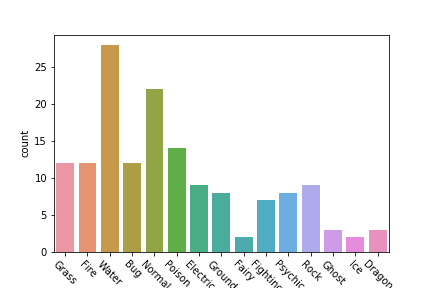
# Count Plot (a.k.a. Bar Plot)
sns.countplot(x='Type 1', data=df)
 
# Rotate x-labels
plt.xticks(rotation=-45)

Line 2: we can use sns.countplot to plot the total count of the categorical variable

第2行：我们可以使用sns.countplot绘制分类变量的总数

Line 5: Using plt.xticks we personalize the graph with a 45⁰ rotation. You should get output like following

第5行：使用plt.xticks我们可以旋转45度来个性化图表。 您应该得到如下输出

When we have categories as columns and numerical value as data then we can use normal barplot as well like following

当我们将类别作为列并将数值作为数据时，我们可以使用普通barplot ，如下所示

sns.barplot(x="Type 1", y="Total", data=df)
plt.xticks(rotation=-45)

使用Seaborn的热图(Heatmap using Seaborn)

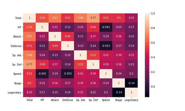
Heatmaps help you visualize matrix-like data. Each cell is color-coded according to its corresponding value. We will check what is the correlation between different columns of the pokemon dataset.

^ h eatmaps帮助您可视化矩阵式的数据。 每个单元格根据其对应的值进行颜色编码。 我们将检查神奇宝贝数据集的不同列之间的相关性。

corr = df.corr()
plt.figure(figsize=(6,6))
sns.heatmap(data=corr, annot=True)

Line 1: df.corr() gives the matrix output of pairwise correlation of columns except for NA values and categorical columns, which is saved in a variable corr

第1行： df.corr()给出除NA值和分类列以外的列的成对相关矩阵输出，该矩阵输出保存在变量corr

Line 2: We set the size of the graph using this plt.figure(figsize=(x,y)) command

第2行：我们使用此plt.figure(figsize=(x,y))命令设置图形的大小

Line 3: we plot the heatplot using this sns.heatplot command. setting annot=True gives the numerical amplitude of correlation along with color-coding.

第3行：我们使用此sns.heatplot命令绘制热图。 设置annot=True给出相关的数值幅度以及颜色编码。

使用Seaborn的散点图 (Scatter plots using Seaborn)

A scatter plot is a type of plot or mathematical diagram using Cartesian coordinates to display values for typically two variables for a set of data. If the points are color-coded, one additional variable can be displayed.

散点图是一种类型的曲线图，或者使用笛卡尔坐标来对一组数据的显示通常是两个变量的值的数学图中。 如果这些点用颜色编码，则可以显示一个附加变量。

sns.scatterplot(x='Attack', y='Defense', data=df, hue='Stage')

Line 1: sns.scatterplot tells the notebook that we want to plot a scatter plot. x-axis, y-axis, and data is given as usual. hue gives color-coding to all the individual data points according to the provided categorical variable Stage

第1行： sns.scatterplot告诉笔记本我们要绘制散点图。 x轴，y轴和数据照常给出。 hue根据提供的分类变量Stage对所有单个数据点进行颜色编码

This data does show some linear regression right? but how can we sure of it? only if there was a way to put fit linear regression lines to the data. And you are in luck my friend, with Seaborn its just one line of code!

这些数据确实显示了线性回归对吗？ 但是我们如何确定呢？ 仅当有办法将拟合线性回归线放入数据中时。 您好运，我的朋友，Seaborn只需一行代码！

sns.lmplot(x='Attack', y='Defense', data=df)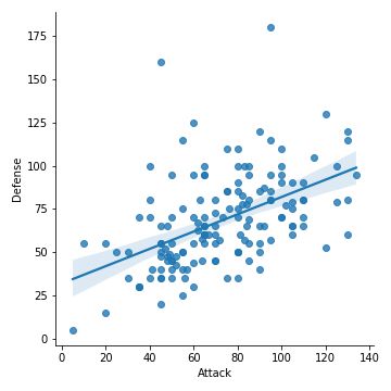

If you want individual regression lines for each value of Stage, then just add hue back in.

如果要为Stage每个值使用单独的回归线，则只需重新添加hue 。

sns.lmplot(x='Attack', y='Defense', data=df, hue="Stage")

A positive slope suggests a positive correlation which can be verified by heatmap as well.

正斜率表示正相关，也可以通过热图验证。

Usually, we use scatter plots to highlight the relationship between two continuous variables (like "heights" and "weights"). However, we can adapt the design of the scatter plot to feature a categorical variable (like "gender") on one of the main axes. and we build it with the sns.swarmplot command.

通常，我们使用散点图突出显示两个连续变量(例如"heights"和"weights" )之间的关系。 但是，我们可以调整散点图的设计，使其在主轴之一上具有分类变量(例如"gender" )。 然后使用sns.swarmplot命令进行构建。

plt.figure(figsize=(12,5))
sns.swarmplot(x='Type 1', y='Attack', data=df)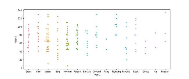

使用Seaborn的直方图(Histograms using Seaborn)

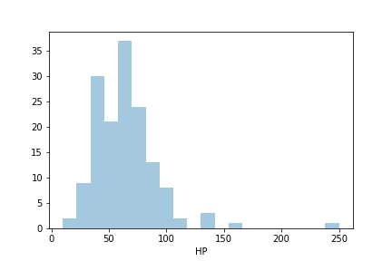
A histogram is an approximate representation of the distribution of numerical data. The higher the height of the bar, the more data falls into the range covered by that bar.

直方图是数值数据的分布的近似表示。 条形图的高度越高，越多的数据落入该条形图覆盖的范围内。

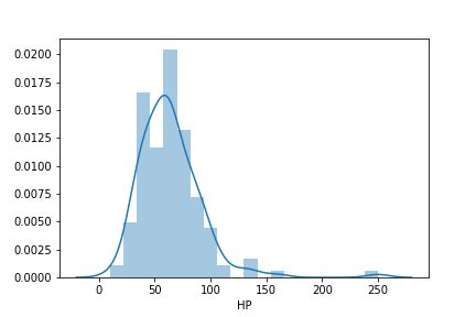
sns.distplot(a=df['HP'], kde=False, bins=20)

Line 1:We use sns.distplot to plot histograms. In the histogram, we dot need to provide x and y as y is by default frequency, so the only input we have to give is a .Note that we do not need to provide an argument data in this command. kde=False removes the kernel density estimation plot on top of the histogram.

第1行：我们使用sns.distplot绘制直方图。 在柱状图，我们点需要提供x和y为y是默认频率，所以我们必须给唯一的输入是a 。注意，我们并不需要提供的参数data在该命令。 kde=False删除直方图顶部的核密度估计图。

kde = False kde = False

kde = True kde =真

We can also print multiple histograms in the same plot just like we did with line plots. Use the same command multiple times with proper input columns.

我们也可以像绘制线图一样在同一图中打印多个直方图。 在正确的输入列中多次使用同一命令。

sns.distplot(a=df['Speed'], label="Speed",kde=False)
sns.distplot(a=df['HP'], label="HP", kde=False)
plt.legend()

Line 1 and Line 2 are the same as aboveLine 3: Forcing the legends to come on a plot with plt.legend() method

第1行和第2行与上述第3行相同：使用plt.legend()方法将图例强制显示在图上

使用Seaborn的密度图(Density plots using Seaborn)

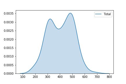
Density plots display the distribution between two variables. One can think of them as a smoothened histogram. They are useful for plotting probability density functions and the probability mass functions of random variables.

d密度曲线显示两个变量之间的分布。 可以将它们视为平滑的直方图。 它们对于绘制随机变量的概率密度函数和概率质量函数很有用。

sns.kdeplot(data=df.Total, shade=True )

Line 1: sns.kdeplot is the command used to plot KDE graph. data is assigned the dataset for plotting and shade=True fills the area under the curve with color.

第1行： sns.kdeplot是用于绘制KDE图的命令。 data分配给绘图数据集，并且shade=True用颜色填充曲线下的区域。

We can also plot multiple KDE plot in the same graph as follows

我们还可以在同一张图中绘制多个KDE图，如下所示

sns.kdeplot(data=df.Total, shade=True )
sns.kdeplot(data=df.HP, shade=True )
sns.kdeplot(data=df.Speed, shade=True )

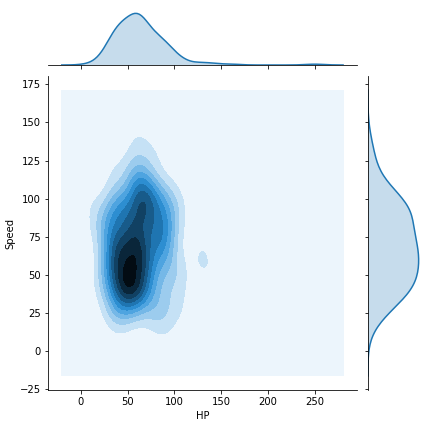
We can also plot 2 column’s KDE plot using sns.jointplot

我们还可以使用sns.jointplot绘制2列的KDE图

sns.jointplot(x="HP", y="Speed", data=df, kind="kde" )

Line 1: Note here that again now we are back to x, y, and data arguments. and kind=”kde” for plotting KDE plot, it is scatter by default.

第1行：请注意，这里我们再次回到x，y和data参数。 和kind=”kde”用于绘制KDE图，默认情况下为scatter 。

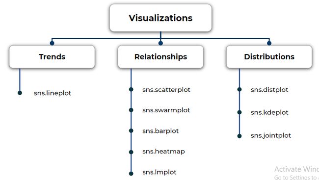
Knowing all this is more than enough to start working with Seaborn. here is the summary of what we learned is in the below image.

了解所有这些，已经足以与Seaborn合作。 这是下图中我们所学的摘要。

You can access the complete jupyter notebook used for this exercise here.

您可以在此处访问用于此练习的完整jupyter笔记本。

Thanks for reading the article! Wanna connect with me?Here is a link to my Linkedin Profile

感谢您阅读本文！ 想与我联系吗？这里是我的Linkedin个人资料的链接

All images are created by the author until given credit

所有图像均由作者创建，直到获得认可为止

Want to learn EDA? follow the article below

想学习EDA吗？ 按照下面的文章

翻译自: https://medium.com/analytics-vidhya/intro-to-data-visualization-using-seaborn-and-matplotlib-6417ecae5abb