RStudio作图
一、准备工作
起初,在进行包的安装操作时,出现了很多错误,通过查找才知道是R的版本不对以及一些包通过现有镜像无法进行下载,所以安装了最新的R版本以及更新了镜像。
镜像:
https://blog.csdn.net/one_time1999/article/details/122368605
R版本:
https://blog.csdn.net/u011262253/article/details/102007737
RStudio生成的图片未出现在对话框中,查找原因才得知是RStudio版本原因,所以更新了最新版本的RStudio。
RStudio版本
https://www.rstudio.com/products/rstudio/download/#download
二、气泡矩阵图
注:
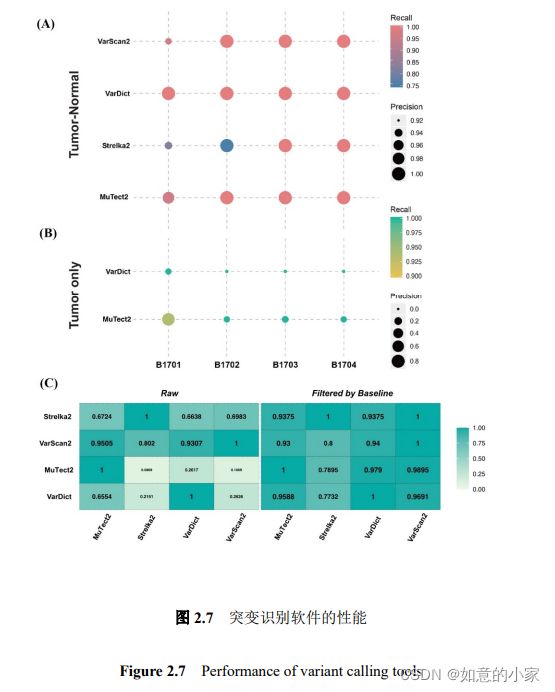
图 2.7(A)表示 VarDict、MuTect2、VarScan2 和 Strelka2 在
Gene Panel 测序的肿瘤-正常配对样本 B1701-B17NC、B1702-B17NC、B1703-B17NC、B1704-B17NC 中的体细胞突变识别的性能。
图 2.7(B)表示两个可用于单肿瘤组织中识别突变的软件 VarDict 和 MuTect2 对样本 B1701、B1702、B1703、B1704 的体细胞突变识别性能。
图中以实心圆点的大小代表软件的准确性,半径越大,软件的准确性越高。实心圆点的颜色代表召回率,颜色越深表示召回率越高。
参考链接:https://www.jianshu.com/p/83724c498199
例子:
文章:https://blog.csdn.net/yangqijia1/article/details/118194934
install.packages("reshape2")
install.packages("ggplot2")

library(reshape2)
library(ggplot2)
data<-read.csv("D:/RStudio/data/tongji_cervical cancer/RNA/Supplementary_Table_51_DEGs_Regression and Normal Tissue.HanXinyin.20181111.v3.csv", header = T)
data<-read.csv("D:/RStudio/data/R_draw_figure/Accuracy_8.csv", header = T)

data#注释:header=T表示数据中的第一行是列名,如果没有列名就用header=F
data_melt<-melt(data,id.vars = "optimizer")#把data中按照“species”的宽数据变成长数据

names(data_melt)=c("optimizer","origin","value")
ggplot(data_melt,aes(x=origin,y=optimizer,size=value,color=origin))+geom_point()+
  theme(panel.background = element_blank(),
        panel.grid = element_line("gray"),
        panel.border = element_rect(colour = "black",fill=NA))

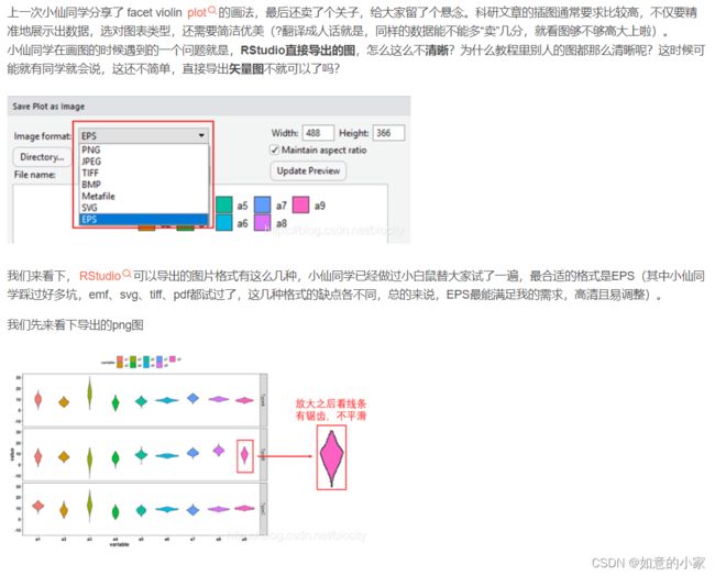
三、RStudio中如何导出高清图
参考连接:https://blog.csdn.net/biocity/article/details/84891289

三、Ai调整画布尺寸大小


四、雷达图
install.packages("reshape2")
install.packages("ggplot2")
library(reshape2)
library(ggplot2)

install.packages("fmsb")
library(fmsb)


#画图:https://www.datanovia.com/en/blog/beautiful-radar-chart-in-r-using-fmsb-and-ggplot-packages/
#bilibili:https://www.bilibili.com/video/av374469972/
#data<-read.csv("D:/RStudio/data/tongji_cervical cancer/RNA/Supplementary_Table_51_DEGs_Regression and Normal Tissue.HanXinyin.20181111.v3.csv", header = T)
data<-read.csv("D:/RStudio/data/R_draw_figure/auc_error.csv", header = T,col.names = c("adam","adamax","SGD","ASGD","RMSprop","Adagrad","Adadelta"),row.names =1)
data
radarfig<-rbind(rep(0,7),rep(1,7),data)
radarfig
rownames(max_min) <- c("Max", "Min")
df <- rbind(max_min, data)
df
student1_data <- df[c("Max", "Min", "cls_test_error"),]
#Basic radar plot
radarchart(student1_data)

# Reduce plot margin using par()
op <- par(mar = c(1, 2, 2, 1))
create_beautiful_radarchart <- function(data, color = "#00AFBB",
                                        vlabels = colnames(data), vlcex = 0.7,
                                        caxislabels = NULL, title = NULL, ...){
  radarchart(
    data, axistype = 1,
    # Customize the polygon
    pcol = color, pfcol = scales::alpha(color, 0.5), plwd = 2, plty = 1,
    # Customize the grid
    cglcol = "grey", cglty = 1, cglwd = 0.8,
    # Customize the axis
    axislabcol = "grey",
    # Variable labels
    vlcex = vlcex, vlabels = vlabels,
    caxislabels = caxislabels, title = title, ...
  )
}
create_beautiful_radarchart(student1_data, caxislabels = c(0, 0.2, 0.4, 0.6, 0.8,1.0))
par(op)


# Reduce plot margin using par()
op <- par(mar = c(1, 2, 2, 2))
# Create the radar charts
create_beautiful_radarchart(
  data = df, caxislabels = c(0, 0.2, 0.4, 0.6, 0.8,1.0),
  color = c("#00AFBB", "#E7B800", "#FC4E07")
)
# Add an horizontal legend
legend(
  x = "bottom", legend = rownames(df[-c(1,2),]), horiz = TRUE,
  bty = "n", pch = 20 , col = c("#00AFBB", "#E7B800", "#FC4E07"),
  text.col = "black", cex = 1, pt.cex = 1.5
)
par(op)

# Define colors and titles
colors <- c("#00AFBB", "#E7B800")
titles <- c("cls_test_error", "cls_auc")

# Reduce plot margin using par()
# Split the screen in 3 parts
op <- par(mar = c(1, 1, 1, 1))
par(mfrow = c(1,2))

# Create the radar chart
for(i in 1:2){
  create_beautiful_radarchart(
    data = df[c(1, 2, i+2), ], caxislabels = c(0, 0.2, 0.4, 0.6, 0.8,1.0),
    color = colors[i], title = titles[i]
  )
}
par(op)
