基于逻辑回归的信用卡欺诈检测

本文是我学习唐宇迪老师的课程做的整理，仅供自己复习。

（一）导入需要使用的包

import pandas as pd
import matplotlib.pyplot as plt
import numpy as np
from sklearn.linear_model import LogisticRegression
from sklearn.model_selection import KFold, cross_val_score  #交叉验证
from sklearn.metrics import confusion_matrix,recall_score,classification_report #混淆矩阵，召回率

%matplotlib inline

（二）读取数据

数据来源：kaggle

data = pd.read_csv("E:\\AAAAAAAAA\\逻辑回归信用卡欺诈检测\\creditcard.csv",engine='python')
data.head()

由于数据涉及隐私，因此每一列的名称没有给出，数据集包含31列，284807个数据，最后一列Class表示类别，0表示正常，1表示欺诈。
（收集数据的方法：

1. 官方网站：kaggle数据集、亚马逊数据集、UCI机器学习数据库、谷歌数据集等
2. 爬虫）

（三）数据预处理

对Amount列进行归一化处理，reshape(-1,1)表示将Amount变成1列，-1表示行数未知；然后去掉‘Time’列和‘Amount’列

from sklearn.preprocessing import StandardScaler

data['normAmount'] = StandardScaler().fit_transform(data['Amount'].reshape(-1, 1))   #列数等于1，行数未知
data = data.drop(['Time','Amount'],axis=1)
data.head()

（四）处理类别不平衡问题

信用卡欺诈毕竟是少数，推断样本可能存在类别不平衡的情况，下面做条状图观察类别的分布情况

count_classes = pd.value_counts(data['Class'], sort = True).sort_index()
count_classes.plot(kind = 'bar')
plt.title("Fraud class histogram")
plt.xlabel("Class")
plt.ylabel("Frequency")

由条状图可以看出，的确存在类别不平衡的情况。类别不平衡的问题通常可以使用欠采样和过采样的方法加以解决。
为什么类别不平衡会影响模型输出?
许多模型的输出类别是基于阈值的，例如逻辑回归中小于0.5的为反例，大于0.5的为正例。在数据类别不平衡时，默认阈值会导致模型输出倾向于类别数据多的类别.
类别不平衡的解决方法：
1）调整阈值，使得模型倾向于类别少的数据；（效果不好）
2）选择合适的评估标准，如ROC曲线或F1值，而不是准确率；
3）欠采样：二分类问题中，假设正例比反例多很多，那么去掉一些正例使得正负比例平衡； （容易出现过拟合问题，泛化能力不强）
4）过采样：二分类问题中，假设正例比反例多很多，那么增加一些负例（重复负例的数据）使得正负比例平衡（容易出现过拟合问题）
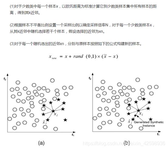
对过采样的改进：SMOTE算法（数据生成策略）

欠采样

X = data.ix[:, data.columns != 'Class']  #样本特征集
y = data.ix[:, data.columns == 'Class']  #样本特征标签

# Number of data points in the minority class（欺诈）
number_records_fraud = len(data[data.Class == 1])
fraud_indices = np.array(data[data.Class == 1].index)

# Picking the indices of the normal classes（正常）
normal_indices = data[data.Class == 0].index

# Out of the indices we picked, randomly select "x" number (number_records_fraud) 
random_normal_indices = np.random.choice(normal_indices, number_records_fraud, replace = False) #随机取number_records_fraud个正常数据
random_normal_indices = np.array(random_normal_indices)

# Appending the 2 indices（合并正常数据和欺诈数据）
under_sample_indices = np.concatenate([fraud_indices,random_normal_indices])

# Under sample dataset（欠采样数据集）
under_sample_data = data.iloc[under_sample_indices,:]

X_undersample = under_sample_data.ix[:, under_sample_data.columns != 'Class']  #欠采样数据集
y_undersample = under_sample_data.ix[:, under_sample_data.columns == 'Class']  #欠采样数据标签
# Showing ratio
print("Percentage of normal transactions: ", len(under_sample_data[under_sample_data.Class == 0])/len(under_sample_data))
print("Percentage of fraud transactions: ", len(under_sample_data[under_sample_data.Class == 1])/len(under_sample_data))
print("Total number of transactions in resampled data: ", len(under_sample_data))

可以看到，数据类别已经达到平衡了。

（五）模型训练

1.划分训练集和测试集

from sklearn.model_selection import train_test_split

# Whole dataset（全集）
X_train, X_test, y_train, y_test = train_test_split(X,y,test_size = 0.3, random_state = 0)  #random_state = 0保证训练集和测试集不变
#X:被划分的样本特征集，y:被划分的样本特征标签
print("Number transactions train dataset: ", len(X_train))
print("Number transactions test dataset: ", len(X_test))
print("Total number of transactions: ", len(X_train)+len(X_test))

# Undersampled dataset（欠采样数据集）
X_train_undersample, X_test_undersample, y_train_undersample, y_test_undersample = train_test_split(X_undersample
                                                                                                   ,y_undersample
                                                                                                   ,test_size = 0.3
                                                                                                   ,random_state = 0)
print("")
print("Number transactions train dataset: ", len(X_train_undersample))
print("Number transactions test dataset: ", len(X_test_undersample))
print("Total number of transactions: ", len(X_train_undersample)+len(X_test_undersample))

2.利用逻辑回归进行模型训练

逻辑回归中有一个重要的参数—正则化项前面的系数C，我们定义一个函数对取不同C值的训练数据集进行5折交叉验证，找到使得召回率最高的C值进行逻辑回归。
召回率（查全率）=TP/（TP+FN）
精度（查准率）=TP/（TP+FP）

def printing_Kfold_scores(x_train_data,y_train_data):
    fold = KFold(5,shuffle=False) 

    # Different C parameters
    c_param_range = [0.01,0.1,1,10,100]   #正则化项前面的系数

    results_table = pd.DataFrame(index = range(len(c_param_range),2), columns = ['C_parameter','Mean recall score'])
    results_table['C_parameter'] = c_param_range

    # the k-fold will give 2 lists: train_indices = indices[0], test_indices = indices[1]
    j = 0
    for c_param in c_param_range:
        print('-------------------------------------------')
        print('C parameter: ', c_param)
        print('-------------------------------------------')
        print('')

        recall_accs = []
        for iteration, indices in enumerate(fold.split(x_train_data):

            # Call the logistic regression model with a certain C parameter
            lr = LogisticRegression(C = c_param, penalty = 'l1')

            # Use the training data to fit the model. In this case, we use the portion of the fold to train the model
            # with indices[0]. We then predict on the portion assigned as the 'test cross validation' with indices[1]
            lr.fit(x_train_data.iloc[indices[0],:],y_train_data.iloc[indices[0],:].values.ravel())

            # Predict values using the test indices in the training data
            y_pred_undersample = lr.predict(x_train_data.iloc[indices[1],:].values)

            # Calculate the recall score and append it to a list for recall scores representing the current c_parameter
            recall_acc = recall_score(y_train_data.iloc[indices[1],:].values,y_pred_undersample)
            recall_accs.append(recall_acc)
            print('Iteration ', iteration,': recall score = ', recall_acc)

        # The mean value of those recall scores is the metric we want to save and get hold of.
        results_table.ix[j,'Mean recall score'] = np.mean(recall_accs)
        j += 1
        print('')
        print('Mean recall score ', np.mean(recall_accs))
        print('')
    results_table['Mean recall score']=results_table['Mean recall score'].astype('float64')
    best_c = results_table.loc[results_table['Mean recall score'].idxmax()]['C_parameter']
    
    # Finally, we can check which C parameter is the best amongst the chosen.
    print('*********************************************************************************')
    print('Best model to choose from cross validation is with C parameter = ', best_c)
    print('*********************************************************************************')
    
    return best_c

best_c = printing_Kfold_scores(X_train_undersample,y_train_undersample)

得到C值为0.01时召回率最大

3.画混淆矩阵（confusion matrix）

def plot_confusion_matrix(cm, classes,
                          title='Confusion matrix',
                          cmap=plt.cm.Blues):
    """
    This function prints and plots the confusion matrix.
    """
    plt.imshow(cm, interpolation='nearest', cmap=cmap)
    plt.title(title)
    plt.colorbar()
    tick_marks = np.arange(len(classes))
    plt.xticks(tick_marks, classes, rotation=0)
    plt.yticks(tick_marks, classes)

    thresh = cm.max() / 2.
    for i, j in itertools.product(range(cm.shape[0]), range(cm.shape[1])):
        plt.text(j, i, cm[i, j],
                 horizontalalignment="center",
                 color="white" if cm[i, j] > thresh else "black")

    plt.tight_layout()
    plt.ylabel('True label')
    plt.xlabel('Predicted label')

import itertools
lr = LogisticRegression(C = best_c, penalty = 'l1')
lr.fit(X_train_undersample,y_train_undersample.values.ravel())
y_pred_undersample = lr.predict(X_test_undersample.values)

# Compute confusion matrix
cnf_matrix = confusion_matrix(y_test_undersample,y_pred_undersample)
np.set_printoptions(precision=2)

print("Recall metric in the testing dataset: ", cnf_matrix[1,1]/(cnf_matrix[1,0]+cnf_matrix[1,1]))

# Plot non-normalized confusion matrix
class_names = [0,1]
plt.figure()
plot_confusion_matrix(cnf_matrix
                      , classes=class_names
                      , title='Confusion matrix')
plt.show()

欠采样数据测试集的混淆矩阵

lr = LogisticRegression(C = best_c, penalty = 'l1')
lr.fit(X_train_undersample,y_train_undersample.values.ravel())
y_pred = lr.predict(X_test.values)

# Compute confusion matrix
cnf_matrix = confusion_matrix(y_test,y_pred)
np.set_printoptions(precision=2)

print("Recall metric in the testing dataset: ", cnf_matrix[1,1]/(cnf_matrix[1,0]+cnf_matrix[1,1]))

# Plot non-normalized confusion matrix
class_names = [0,1]
plt.figure()
plot_confusion_matrix(cnf_matrix
                      , classes=class_names
                      , title='Confusion matrix')
plt.show()

全部数据测试集的混淆矩阵

可以看到，召回率比较高，但是存在12570个原本是正常被五分为诈骗的，精度比较低。
上面都是基于欠采样数据训练集进行模型训练，下面基于全部数据进行训练。
基于全部数据集的训练

best_c = printing_Kfold_scores(X_train,y_train)

lr = LogisticRegression(C = best_c, penalty = 'l1')
lr.fit(X_train,y_train.values.ravel())
y_pred_undersample = lr.predict(X_test.values)

# Compute confusion matrix
cnf_matrix = confusion_matrix(y_test,y_pred_undersample)
np.set_printoptions(precision=2)

print("Recall metric in the testing dataset: ", cnf_matrix[1,1]/(cnf_matrix[1,0]+cnf_matrix[1,1]))

# Plot non-normalized confusion matrix
class_names = [0,1]
plt.figure()
plot_confusion_matrix(cnf_matrix
                      , classes=class_names
                      , title='Confusion matrix')
plt.show()

可以看到，在全部数据的测试集上，召回率只有0.619，比较低。由此可以看出欠采样方法确实存在一些问题。

不同分类阈值下的混淆矩阵

lr = LogisticRegression(C = 0.01, penalty = 'l1')
lr.fit(X_train_undersample,y_train_undersample.values.ravel())
y_pred_undersample_proba = lr.predict_proba(X_test_undersample.values)

thresholds = [0.1,0.2,0.3,0.4,0.5,0.6,0.7,0.8,0.9]  #0.1表示大于0.1预测为1，小于0.1预测为0，以此类推

plt.figure(figsize=(10,10))

j = 1
for i in thresholds:
    y_test_predictions_high_recall = y_pred_undersample_proba[:,1] > i
    
    plt.subplot(3,3,j)
    j += 1
    
    # Compute confusion matrix
    cnf_matrix = confusion_matrix(y_test_undersample,y_test_predictions_high_recall)
    np.set_printoptions(precision=2)

    print("Recall metric in the testing dataset: ", cnf_matrix[1,1]/(cnf_matrix[1,0]+cnf_matrix[1,1]))

    # Plot non-normalized confusion matrix
    class_names = [0,1]
    plot_confusion_matrix(cnf_matrix
                          , classes=class_names
                          , title='Threshold >= %s'%i) 

4.过采样（SMOTE）

import pandas as pd
from imblearn.over_sampling import SMOTE
from sklearn.ensemble import RandomForestClassifier
from sklearn.metrics import confusion_matrix
from sklearn.model_selection import train_test_split

credit_cards=pd.read_csv("E:\\AAAAAAAAA\\逻辑回归信用卡欺诈检测\\creditcard.csv",engine='python')

columns=credit_cards.columns
# The labels are in the last column ('Class'). Simply remove it to obtain features columns
features_columns=columns.delete(len(columns)-1)

features=credit_cards[features_columns]
labels=credit_cards['Class']

features_train, features_test, labels_train, labels_test = train_test_split(features, 
                                                                            labels, 
                                                                            test_size=0.2, 
                                                                            random_state=0)

oversampler=SMOTE(random_state=0)
os_features,os_labels=oversampler.fit_sample(features_train,labels_train)
len(os_labels[os_labels==1])   #227454

os_features = pd.DataFrame(os_features)
os_labels = pd.DataFrame(os_labels)
best_c = printing_Kfold_scores(os_features,os_labels)

lr = LogisticRegression(C = best_c, penalty = 'l1')
lr.fit(os_features,os_labels.values.ravel())
y_pred = lr.predict(features_test.values)

# Compute confusion matrix
cnf_matrix = confusion_matrix(labels_test,y_pred)
np.set_printoptions(precision=2)

print("Recall metric in the testing dataset: ", cnf_matrix[1,1]/(cnf_matrix[1,0]+cnf_matrix[1,1]))

# Plot non-normalized confusion matrix
class_names = [0,1]
plt.figure()
plot_confusion_matrix(cnf_matrix
                      , classes=class_names
                      , title='Confusion matrix')
plt.show()

可以看到召回率要比欠采样小一些，但模型的精度变高了。过采样的整体效果更好。一般情况下采用过采样。