金融风控实战——逻辑回归与评分卡模型（上）

评分卡

• 建立逻辑回归模型
• 对模型进行评分映射

逻辑回归表达式

import numpy as np
import matplotlib.pyplot as plt
import tqdm
import os
data = np.loadtxt("/Users/zhucan/Desktop/金融风控实战/第五课资料/textSet.txt")
features = data[:, :2]
labels = data[:, -1]
print(features.shape, labels.shape)
#(100, 2) (100,)
print('特征的维度: {0}'.format(features.shape[1]))
print('总共有{0}个类别'.format(len(np.unique(labels))))
#特征的维度: 2
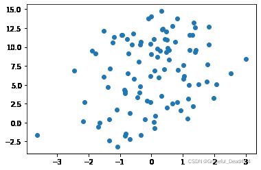
#总共有2个类别

#可视化
plt.scatter([x[0] for x in features], [x[1] for x in features])
plt.show()

结果： 

sigmoid函数 

def sigmoid(x):
    return  1 / (1 + np.exp(-x))
print(sigmoid(-5), sigmoid(5))
#0.0066928509242848554 0.9933071490757153

sigmoid函数的导数 

def delta_sigmoid(x):
    return sigmoid(x) * (1 - sigmoid(x))
delta_sigmoid(5)
#0.006648056670790033

基础建模

随机初始化权重, 从正态分布中生成

W = np.random.uniform(size=(1, features.shape[1]))
W
#array([[0.20881179, 0.53058372]])

矩阵乘法

def matrix_mul(matrix1, matrix2):
    return np.matmul(matrix1, matrix2)
print(matrix_mul(np.random.uniform(size=(1, 2)), np.random.uniform(size=(2, 1))))
#[[0.71085393]]

矩阵求导 

def delta_matrix(X, W):
    return np.matmul(X.T, np.ones(shape=(len(X), 1))).T / len(X)
W = np.random.uniform(low=0, high=1, size=(1, 2))
X = np.random.uniform(low=3, high=15, size=(3, 2))
delta = delta_matrix(X, W)
print(delta, W - delta)
#[[13.51261268  7.53774522]] [[-12.86444081  -7.16950368]]

包含偏置项 

def add_bias(result, B):
#     assert len(result) == len(B)
    return result + B
B = np.random.uniform(size=(1,))
print(B, add_bias(matrix_mul(W, X.T), B))
#[0.07422123] [[ 7.97809996 13.6316383  13.87457563]]

对偏置项求导

def delta_B():
    return 1
delta_B()
#1

完整的逻辑回归 inference 

def logic(W, X, B):
    mul = matrix_mul(W, X)
    y = add_bias(mul, B)
    return y
logic(W, X.T, B)
#array([[ 7.97809996, 13.6316383 , 13.87457563]])

损失函数(Cross-entropy, 交叉熵损失函数) 

信息熵: −(P是概率, 小于1, 取反之后就是正数了), 这个值代表的是信息量, 如果值越大代表对当前情况越不确定, 信息不足.

def loss(Y_t, Y_p):
    '''
        算交叉熵损失函数
        Y_t: 独热编码之后的真实值向量
        Y_p: 预测的值向量        
    '''
    trans = np.zeros(shape=Y_t.shape)
    for sample_idx in range(len(trans)):
        # print(trans[sample_idx], [Y_p[sample_idx], 1.0 - Y_p[sample_idx]])
        # 避免出现0
        trans[sample_idx] = [Y_p[0][sample_idx] , 1.0 - Y_p[0][sample_idx] + 1e-5]
    log_y_p = np.log(trans)
    return -np.sum(np.multiply(Y_t, log_y_p))
Y_t = np.array([[0, 1], [1, 0]])
Y_p = np.array([[0.8, 1]])
loss(Y_t=Y_t, Y_p=Y_p)
#1.609387913684059

交叉熵求导 

def delta_cross_entropy(Y_t, Y_p):
    trans = np.zeros(shape=Y_t.shape)
    for sample_idx in range(len(trans)):
        trans[sample_idx] = [Y_p[0][sample_idx] + 1e-8, 1.0 - Y_p[0][sample_idx] + 1e-8]
    Y_t[Y_t == 0] += 1e-8
    error = Y_t * (1 / trans)
    error[:, 0] = -error[:, 0]
    return np.sum(error, axis=1, keepdims=True)
Y_t = np.array([[0, 1], [1, 0]], dtype=np.float)
Y_p = np.array([[0.8, 1]])
delta_cross_entropy(Y_t=Y_t, Y_p=Y_p)
#array([[4.99999974e+00],
#      [9.99999983e-09]])

准确率计算

def accuracy(Y_p, Y_t):
    Y_p[Y_p >= 0.5] = 1
    Y_p[Y_p < 0.5] = 0
    predict = np.sum(Y_p == Y_t)
    return predict /  len(Y_t)

评估指标

def recall(Y_p, Y_t):
    return np.sum(np.argmax(Y_p) == np.argmax(Y_t)) / np.sum(Y_p == 1)

独热编码

如果有两个类别

def one_hot(y):
    classes = np.arange(len(np.unique(y)))
    one_hot_label = np.zeros(shape=(len(y), len(classes)))
    for sample in range(len(y)):
        one_hot_label[sample][classes == y[sample]] = 1
    return one_hot_label

one_hot([0, 1, 2, 3])

结果：

array([[1., 0., 0., 0.],
       [0., 1., 0., 0.],
       [0., 0., 1., 0.],
       [0., 0., 0., 1.]])

更新权重 

def update_parameters(Y_t, W, B, X, learning_rate=0.1):
#     mul = matrix_mul(W, X)
#     Y_p = add_bias(mul, B)
    Y_p = np.matmul(W, X.T)
    Y_p += B
    Y_p = sigmoid(Y_p)
    error = loss(one_hot(Y_t), Y_p)
    # 里面是按列计算的, 进行了转换, 所以这里也需要转置
#     delta_loss = delta_cross_entropy(one_hot(Y_t), Y_p)
    
#     delta_activation = delta_sigmoid(Y_p)
#     derror = np.multiply(delta_loss, delta_activation)
#     dw = np.matmul(derror, X)
    # 误差项
    error_rate = Y_p - Y_t
    deltaW = np.matmul(error_rate, X) / len(Y_t)
    deltaB = error_rate * delta_B()
    deltaB = np.sum(deltaB) / len(X)
    W -= (learning_rate * deltaW)
    B -= (learning_rate * deltaB)
    return error, W, B

np.random.seed(1)
W = np.random.uniform(size=(1, 2))
print(W)
X = np.random.uniform(size=(3, 2))
Y_t = np.array([1, 0, 1])
update_parameters(Y_t, W, B, X)
#[[0.417022   0.72032449]]
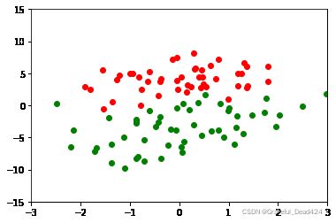
#(2.360515176075121, array([[0.41682199, 0.72755927]]), array([0.08349814]))

归一化特征数据并且可视化 

import copy

def normalize(x, mean, max_value, min_value, is_normalize=False):
    f = copy.deepcopy(x)
    f -= mean
    if is_normalize:
        f = (f - min_value) / (max_value - min_value)
    return f

mean = np.mean(features, axis=0)
max_value = np.max(features, axis=0)
min_value = np.min(features, axis=0)

f_normalize_features = normalize(features, mean, max_value, min_value)

figure = plt.figure()
plt.scatter([x[0] for x in f_normalize_features[labels == 0]], [x[1] for x in f_normalize_features[labels == 0]], c='r')
plt.scatter([x[0] for x in f_normalize_features[labels == 1]], [x[1] for x in f_normalize_features[labels == 1]], c='g')
plt.xlim(left=-3, right=3)
plt.ylim(bottom=-15, top=15)
plt.show()

结果： 

mean = np.mean(features, axis=0)
max_value = np.max(features, axis=0)
min_value = np.min(features, axis=0)

f_normalize_features = normalize(features, mean, max_value, min_value, is_normalize=True) 
#is_normalize为True

figure = plt.figure()
plt.scatter([x[0] for x in f_normalize_features[labels == 0]], [x[1] for x in f_normalize_features[labels == 0]], c='r')
plt.scatter([x[0] for x in f_normalize_features[labels == 1]], [x[1] for x in f_normalize_features[labels == 1]], c='g')
plt.xlim(left=-1, right=2)
plt.ylim(bottom=-2, top=2)
plt.show()

 结果：
拆分数据集

分为训练集和测试集, 占比为0.7:0.3

test_size = int(len(labels) * 0.3)
random_idx = np.random.permutation(len(labels))
test_features = features[random_idx[:test_size]]
test_labels = labels[random_idx[:test_size]]
train_features = features[random_idx[test_size:]]
train_labels = labels[random_idx[test_size:]]

print('test_features type{0}'.format(test_features.shape))
print('train_features type{0}'.format(train_features.shape))
#test_features type(30, 2)
#train_features type(70, 2)

推理加训练 

## 学习的曲线
def drawLine(weights, B=0):
    dataArr = features
    n = np.shape(dataArr)[0] 
    xcord1 = []; ycord1 = []
    xcord2 = []; ycord2 = []
    for i in range(n):
        if int(labels[i])== 1:
            xcord1.append(dataArr[i,0]); ycord1.append(dataArr[i,1])
        else:
            xcord2.append(dataArr[i,0]); ycord2.append(dataArr[i,1])
    fig = plt.figure()
    ax = fig.add_subplot(111)
    ax.scatter(xcord1, ycord1, s=30, c='red', marker='s')
    ax.scatter(xcord2, ycord2, s=30, c='green')
    x = np.arange(-3.0, 3.0, 0.1)
    y = (-B-weights[0][1]*x-1) / weights[0][1]
    ax.plot(x, y)
    plt.xlabel('X1'); plt.ylabel('X2');
    plt.show()
def train(train_features, test_features, train_labels, test_labels, epoch=15, learning_rate=0.008):
    W = np.random.uniform(size=(1, train_features.shape[1]))
    B = 0
    for current in range(epoch):
        np.random.seed(current)
        random_train_features_idx = np.random.choice(np.arange(len(train_features)), size=(16,))
        random_train_features = train_features[random_train_features_idx]
        random_train_labels = train_labels[random_train_features_idx]
        print('Update W:', W)
        Y_p = np.matmul(W, train_features.T)
        Y_p += B
        Y_p = sigmoid(Y_p)
        error = loss(one_hot(train_labels), Y_p) / len(random_train_features)
        # 误差项
        error_rate = Y_p - train_labels
        deltaW = np.matmul(error_rate, train_features) / len(random_train_labels)
        deltaB = error_rate * delta_B()
        deltaB = np.sum(deltaB) / len(random_train_labels)
        W -= (learning_rate * deltaW)
        B -= (learning_rate * deltaB)
        print('epoch {0}: train_loss:{1}'.format(current + 1, error))
        drawLine(W, B)
    return W, B
train(train_features, test_features, train_labels, test_labels)

结果：