人工智能实践Tensorflow2.0 第四章--1.增强八股搭建神经网络--北京大学慕课

第四章–增强八股搭建神经网络
本讲目标：
  用增强八股搭建神经网络。参考视频。

0.回顾八股

0.1-回顾六步法

①import
②train,test
  这一步要学习自制数据集，符合自己行业领域的数据。另外学习数据增强。
③model=tf.keras.Sequantial
④model.compile
⑤model.fit
  这一步学习断点续训，可以再上一次训练的结果上接着训练。
⑥model.summary
  这一步学习参数提取，可以将训练好的参数提取出来，作为移植到其他平台使用。学习acc/loss可视化，可以很好的分析结果。

1.数据增强，扩充数据集

  数据增强可以帮助扩展数据集，数据增强就是对图像的简单形变，用来应对因拍照角度问题带来的图片变形。Tensorflow给出了数据增强函数，只需要给定数据增强的方式及参数即可。

1.1-API: tf.keras.preprocessing.image.ImageDataGenerator

image_gen_train=tf.keras.preprocessing.image.ImageDataGenerator(
rescale = 所有数据将乘以该数值,
rotation_range = 随机旋转角度数范围,
width_shift_range = 随机宽度偏移量,
height_shift_range = 随机高度偏移量,
horizontal_flip = 是否随机水平翻转,
zoom_range =  随机缩放的范围 [1-n ，1+n] 
)
image_gen_train.fit(x_train)

例如：

image_gen_train = ImageDataGenerator(
rescale=1. / 255,     # 将图像数据归为0~1
rotation_range=45,   # 随机45度旋转
width_shift_range=.15, # 宽度偏移
height_shift_range=.15, # 高度偏移
horizontal_flip=False,  # 水平翻转
zoom_range=0.5     # 将图像随机缩放阈量50％
)
image_gen_train.fit(x_train)

注：
1. 数据增强要求数据的格式为四维，故扩充一维度即可。

x_train = x_train.reshape(x_train.shape[0], 28, 28, 1) (60000, 28, 28) =>(60000, 28, 28, 1) 2. 调用数据增强之后的数据方法为 model.fit(x_train, y_train,batch_size=32, ……) ↓ model.fit(image_gen_train.flow(x_train,y_train,batch_size=32), ……)

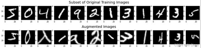
1.2-数据增强可视化

import tensorflow as tf
from tensorflow.keras.preprocessing.image import  ImageDataGenerator
import matplotlib.pyplot as plt
import numpy as np

(x_train,y_train),(x_test,y_test)=tf.keras.datasets.mnist.load_data()
print(x_train.shape)
print(y_train.shape)
print(x_test.shape)
print(y_test.shape)
x_train,x_test=x_train/255.0,x_test/255.0
x_train=x_train.reshape(x_train.shape[0],28,28,1)#给数据增加一个维度，从(60000,28,28)reshape为(60000,28,28,1)

image_gen_train=ImageDataGenerator(
    rescale=1./1.,#如为图像，分母为255时，可归一化至0~1
    rotation_range=45,#随机旋转45°
    width_shift_range=.15,#宽度偏移
    height_shift_range=.15,#高度偏移
    horizontal_flip=False,#水平翻转
    zoom_range=0.5#将图像随机缩放阈量50%
)
image_gen_train.fit(x_train)
print('x_train',x_train.shape)
x_train_subset1=np.squeeze(x_train[:12])
print('x_train_subset1',x_train_subset1.shape)
print('x_train',x_train.shape)
x_train_subset2=x_train[:12]
print('x_train_subset2',x_train_subset2.shape)

fig=plt.figure(figsize=(20,2))
plt.set_cmap('gray')
#显示原始图片
for i in range(0,len(x_train_subset1)):
    ax=fig.add_subplot(1,12,i+1)
    ax.imshow(x_train_subset1[i])
fig.suptitle('Subset of Original Training Images', fontsize=20)
plt.show()

#增强后的照片
fig=plt.figure(figsize=(20,2))
for x_batch in image_gen_train.flow(x_train_subset2,batch_size=12,shuffle=False):
    for i in  range(0,12):
        ax=fig.add_subplot(1,12,i+1)
        ax.imshow(np.squeeze(x_batch[i]))
    fig.suptitle("Augmented Images",fontsize=20)
    plt.show()

输出结果如下：

(60000, 28, 28)
(60000,)
(10000, 28, 28)
(10000,)
x_train (60000, 28, 28, 1)
x_train_subset1 (12, 28, 28)
x_train (60000, 28, 28, 1)
x_train_subset2 (12, 28, 28, 1)

2.断点续训，存取模型

  断点续训可用于保存训练的模型，在下次训练时可加载已经训练好的模型继续训练。

2.1-读取模型

load_weights( 路径文件名)

---

#定义保存模型的路径
checkpoint_save_path = "./checkpoint/mnist.ckpt"
#如果该路径中存在模型，则加载
if os.path.exists(checkpoint_save_path + '.index'):
    print('-------------load the model-----------------')
    model.load_weights(checkpoint_save_path)

---

2.2-保存模型

---

tf.keras.callbacks.ModelCheckpoint(
filepath=路径文件名 ,
save_weights_only=True/False,是否只保存权重
save_best_only= True/False，是否只保存最好的结果
) 

---

回调函数要加入fit当中

history = model.fit（callbacks=[cp_callback] ）

---

#定义保存模型的路径
checkpoint_save_path = "./checkpoint/mnist.ckpt"
#如果该路径中存在模型，则加载
if os.path.exists(checkpoint_save_path + '.index'):
    print('-------------load the model-----------------')
    model.load_weights(checkpoint_save_path)
#定义保存模型的回调函数
cp_callback = tf.keras.callbacks.ModelCheckpoint(filepath=checkpoint_save_path,
                          save_weights_only=True,
                          save_best_only=True)
#在训练时加入保存模型的回调函数
history = model.fit(x_train, y_train, batch_size=32, epochs=5, validation_data=(x_test, y_test), validation_freq=1,
                    callbacks=[cp_callback])

---

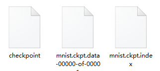
生成三个文件如下，即为保存模型。

---

3.参数提取

  可以把训练好的参数读入文本。

3.1-设置输出格式：np.set_pointoptions

---

np.set_printoptions (
 precision=小数点后按四舍五入保留几位,
 threshold=数组元素数量少于或等于门槛值，打印全部元素；否则打印门槛值+1 个元素，中间用省略号补充)
例如：

threshold=5,      打印5+1=6个元素
threshold=np.inf,  打印全部元素
precision=np.inf,  打印完整小数

---

#打印保留小数点后5位
np.set_printoptions(precision=5)
print(np.array([1.123456789]))
[1.12346]

#打印只显示6个元素，其余用省略号代替
np.set_printoptions(threshold=5)
print(np.arange(10))
[0 1 2 ... 7 8 9]

#打印全部元素
np.set_printoptions(threshold=np.inf)
print(np.arange(10))
[0 1 2 3 4 5 6 7 8 9]

---

3.2-提取可训练参数：model.trainable_variables

---

  model.trainable_variables 返回模型中可训练的参数

print(model.trainable_variables)
file = open('./weights.txt', 'w')
for v in model.trainable_variables:
    file.write(str(v.name) + '\n')
    file.write(str(v.shape) + '\n')
    file.write(str(v.numpy()) + '\n')
file.close()

---

4.acc/loss可视化，查看训练效果

4.1-acc曲线与loss曲线

history=model.fit (
  train_data, train_label,
  batch_size= , epochs= ,
  validation_data=(test_data,test_label),
  validation_split=从训练集划分多少比例给测试集，
  validation_freq = 多少个epoch 测试一次
)
history:

训练集损失： loss
测试集损失： val_loss
训练集准确率： sparse_categorical_accuracy
测试集准确率： val_sparse_categorical_accuracy

---

# 显示训练集和验证集的acc和loss曲线
acc = history.history['sparse_categorical_accuracy']
val_acc = history.history['val_sparse_categorical_accuracy']
loss = history.history['loss']
val_loss = history.history['val_loss']

plt.subplot(1, 2, 1)
plt.plot(acc, label='Training Accuracy')
plt.plot(val_acc, label='Validation Accuracy')
plt.title('Training and Validation Accuracy')
plt.legend()

plt.subplot(1, 2, 2)
plt.plot(loss, label='Training Loss')
plt.plot(val_loss, label='Validation Loss')
plt.title('Training and Validation Loss')
plt.legend()
plt.show()

---

5-完整代码

---

##六步法第一步->import导入需要的包
import tensorflow as tf
import os
import numpy as np
from matplotlib import pyplot as plt

np.set_printoptions(threshold=np.inf)
##六步法第二步->加载train和test
mnist = tf.keras.datasets.mnist
(x_train, y_train), (x_test, y_test) = mnist.load_data()
x_train, x_test = x_train / 255.0, x_test / 255.0
##六步法第三步->搭建网络Model
model = tf.keras.models.Sequential([
    tf.keras.layers.Flatten(),
    tf.keras.layers.Dense(128, activation='relu'),
    tf.keras.layers.Dense(10, activation='softmax')
])
##六步法第四步->compile配置网络
model.compile(optimizer='adam',
              loss=tf.keras.losses.SparseCategoricalCrossentropy(from_logits=False),
              metrics=['sparse_categorical_accuracy'])
##加入断点续训，可以读取之前保存的网络，如果之前没有保存，则不读取
checkpoint_save_path = "./checkpoint/mnist.ckpt"
if os.path.exists(checkpoint_save_path + '.index'):
    print('-------------load the model-----------------')
    model.load_weights(checkpoint_save_path)
# 断点续训的保存网络的回调函数
cp_callback = tf.keras.callbacks.ModelCheckpoint(filepath=checkpoint_save_path,
                          save_weights_only=True,
                          save_best_only=True)
##六步法第五步->fit训练网络
history = model.fit(x_train, y_train, batch_size=32, epochs=5, validation_data=(x_test, y_test), validation_freq=1,
                    callbacks=[cp_callback])
##六步法第六步->summary查看网络
model.summary()

#打印可训练参数
print(model.trainable_variables)
file = open('./weights.txt', 'w')
for v in model.trainable_variables:
    file.write(str(v.name) + '\n')
    file.write(str(v.shape) + '\n')
    file.write(str(v.numpy()) + '\n')
file.close()

###############################################    show   ###############################################

# 显示训练集和验证集的acc和loss曲线
acc = history.history['sparse_categorical_accuracy']
val_acc = history.history['val_sparse_categorical_accuracy']
loss = history.history['loss']
val_loss = history.history['val_loss']

plt.subplot(1, 2, 1)
plt.plot(acc, label='Training Accuracy')
plt.plot(val_acc, label='Validation Accuracy')
plt.title('Training and Validation Accuracy')
plt.legend()

plt.subplot(1, 2, 2)
plt.plot(loss, label='Training Loss')
plt.plot(val_loss, label='Validation Loss')
plt.title('Training and Validation Loss')
plt.legend()
plt.show()

---

6.应用程序，给图识物

  前向传播执行应用。
model.predict(输入特征, batch_size=整数),返回前向传播计算结果。

---

###复现模型###
model=tf.keras.models.Sequential(
    [
     tf.keras.layers.Flatten(),
     tf.keras.layres.Dense(128,activation='relu'),
     tf.keras.layers.Dense(10,activation='softmax')
    ]
)
###加载参数###
model.load_weights(model_save_path)
###预测结果###
result=model.predict(x_predict)


***************************************************************
from PIL import  Image
import  numpy as np
import  tensorflow as tf
###加载模型参数###
model_save_path='./checkpoint/mnist.ckpt'

###复现模型###
model=tf.keras.Sequential([
    tf.keras.layers.Flatten(),
    tf.keras.layers.Dense(128,activation='relu',kernel_regularizer=tf.keras.regularizers.l2()),
    tf.keras.layers.Dense(10,activation='softmax')
])

###加载权重###
model.load_weights(model_save_path)

##预测模型###
#预测图片的数量
perNum=int(input('input the number of test pictures:'))
for i in range(perNum):
    #预测图片的路径
    image_path=input("the path of the pictures")
    img=Image.open(image_path)#打开图片
    img=img.resize((28,28),Image.ANTIALIAS)#调整尺寸
    img_arr=np.array(img.convert('L'))
    #二值化图片
    for i in range(28):
        for j in range(28):
            if img_arr[i][j]<200:
                img_arr[i][j]=255
            else:
                img_arr[i][j]=0
    img_arr=img_arr/255.
    #预测结果
    x_predict=img_arr[tf.newaxis,...]
    result=model.predict(x_predict)
    pred=tf.argmax(result,axis=1)
    print('\n')
    tf.print(pred)

---

注：
  输出结果pred是张量，需要用tf.print才可以打印。打印出来的结果‘3’，输出为：
tf.Tensor([3],shape=(1,), dtype=int64)