Opencv学习笔记(十二)图像几何变换
文章目录
-
- 代码
图像的几何变换包括图像缩放、平移、旋转、仿射变换、透视变换。
代码
import cv2
import numpy as np
from matplotlib import pyplot as plt
src1 = cv2.imread(r'F:\OPENCV\Opencv\flower.jfif', cv2.IMREAD_COLOR)
src2 = cv2.imread(r'F:\OPENCV\Opencv\test4.png', cv2.IMREAD_COLOR)
src = cv2.cvtColor(src1, cv2.COLOR_BGR2RGB)
src0 = cv2.cvtColor(src2, cv2.COLOR_BGR2RGB)
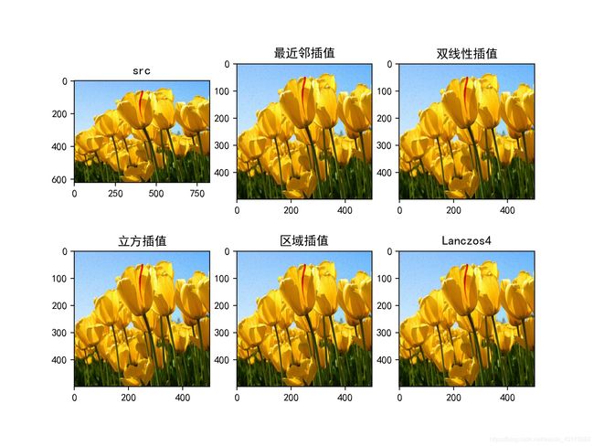
# 图像缩放
# cv2.resize(src, size, fx, fy, interpolation),参数依次为原始图片大小、缩放大小、x方向缩放因子、y方向缩放因子、插值方法.
img1 = cv2.resize(src, (500, 500), cv2.INTER_NEAREST) # 最近邻插值
img2 = cv2.resize(src, (500, 500), cv2.INTER_LINEAR) # 双线性插值(默认使用)
img3 = cv2.resize(src, (500, 500), cv2.INTER_CUBIC) # 立方插值(耗时)
img4 = cv2.resize(src, (500, 500), cv2.INTER_AREA) # 区域插值(图像缩小时推荐使用)
img5 = cv2.resize(src, (500, 500), cv2.INTER_LANCZOS4) # Lanczos4插值(8*8邻域插值算法)
# 显示各个图像
plt.rcParams['font.sans-serif'] = ['SimHei']
titles = ['src', '最近邻插值', '双线性插值', '立方插值', '区域插值', 'Lanczos4']
images = [src, img1, img2, img3, img4, img5]
plt.figure(1, figsize=(6, 6))
for i in range(len(images)):
plt.subplot(2, 3, i + 1)
plt.imshow(images[i], 'gray')
plt.title(titles[i])
plt.xticks([])
plt.yticks([])
plt.savefig(r'F:\OPENCV\Opencv\flower.jpg', dpi=200)
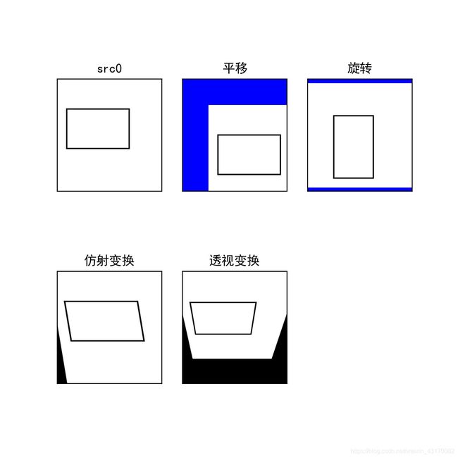
# 平移
# 构建平移矩阵, 数据类型为浮点型
# M = np.float32([[1, 0, 100],
# [0, 1, 100]])
M1 = np.array([[1, 0, 100],
[0, 1, 100]]).astype(np.float)
# cv2.warpAffine(),M1为平移矩阵,(src.shape[1], src.shape[0])为输出图像大小
translation = cv2.warpAffine(src0, M1, (src0.shape[1], src0.shape[0]),
borderMode=cv2.BORDER_CONSTANT, borderValue=[0, 0, 255])
# 旋转
# (src0.shape[1] / 2, src0.shape[0] / 2)为图像中心点, angle为旋转角度, scale为缩放因子
M2 = cv2.getRotationMatrix2D((src0.shape[1] / 2, src0.shape[0] / 2), angle=90, scale=1)
print(M1)
dst = cv2.warpAffine(src0, M2, (src0.shape[1], src0.shape[0]),
borderMode=cv2.BORDER_CONSTANT, borderValue=[0, 0, 255])
# 仿射变换,保持图像中的平行关系。
points1 = np.float32([[40, 40],
[160, 40],
[40, 160]])
points2 = np.float32([[20, 40],
[160, 40],
[40, 160]])
# points1, points2分别为原始图像、目标图像中的对应的点。、
# cv2.getAffineTransform()返回一个2*3的矩阵。
M3 = cv2.getAffineTransform(points1, points2)
dst1 = cv2.warpAffine(src0, M3, (src0.shape[1], src0.shape[0]))
# 透视变换,目的是变换前后图像中的直线依然是直线。
points3 = np.float32([[40, 40],
[160, 40],
[40, 160],
[160, 160]])
points4 = np.float32([[20, 40],
[160, 40],
[40, 160],
[160, 160]])
# points3, points4分别为原始图像、目标图像中的对应的点(不共线)。
# cv2.getPerspectiveTransform()返回一个3*3的矩阵。
M4 = cv2.getPerspectiveTransform(points3, points4)
# cv2.warpPerspective()透视变换函数
dst2 = cv2.warpPerspective(src0, M4, (src0.shape[1], src0.shape[0]))
# 显示图像
titles1 = ['src0', '平移', '旋转', '仿射变换', '透视变换']
images1 = [src0, translation, dst, dst1, dst2]
plt.figure(2, figsize=(6, 6))
for i in range(len(images1)):
plt.subplot(2, 3, i + 1)
plt.imshow(images1[i], 'gray')
plt.title(titles1[i])
plt.xticks([])
plt.yticks([])
plt.show()
结果图像