天池龙珠数据挖掘训练营 Task4 学习笔记(建模调参)
天池龙珠数据挖掘训练营学习笔记
- 天池龙珠数据挖掘训练营 Task1 学习笔记(赛题理解)
- 天池龙珠数据挖掘训练营 Task2 学习笔记(数据分析)
- 天池龙珠数据挖掘训练营 Task3 学习笔记(特征工程)
- 天池龙珠数据挖掘训练营 Task4 学习笔记(建模调参)
- 天池龙珠数据挖掘训练营 Task5 学习笔记(模型融合)
- 天池龙珠数据挖掘训练营 Task6 学习笔记(二手车交易价格预测)
文章目录
- 天池龙珠数据挖掘训练营学习笔记
- 前言
- 一、学习知识点概要
- 二、学习内容
-
- 0 各种模型的原理
- 1 读取处理好的数据
- 2 线性回归 & 五折交叉验证 & 模拟真实业务情况
-
- 2.1 简单建模
- 2.2 五折交叉验证
- 2.3 模拟真实业务情况
- 2.4 绘制学习率曲线与验证曲线
- 3 多种模型对比
-
- 3.1 线性模型 & 嵌入式特征选择
- 3.2 非线性模型
- 4 模型调参
-
- 4.1 贪心调参
- 4.2 Grid Search 调参
- 4.3 贝叶斯调参
- 学习问题与解答
-
-
- 问题1 :简单建模后需要可视化所有特征吗
- 问题2 : 调参神器贝叶斯优化(bayesian-optimization)
-
- 学习思考与总结
前言
有了前面的数据处理后,本节开始建模调参。
通过本节的学习,基本了解常用的机器学习模型,并掌握机器学习模型的建模与调参流程。
一、学习知识点概要
- 线性回归模型
- 模型性能验证
- 嵌入式特征选择
- 模型对比
- 模型调参
二、学习内容
0 各种模型的原理
- 略
1 读取处理好的数据
import pandas as pd
import numpy as np
import warnings
warnings.filterwarnings('ignore')
- 优化
reduce_mem_usage 函数通过调整数据类型,减少数据在内存中占用的空间
def reduce_mem_usage(df):
    """ iterate through all the columns of a dataframe and modify the data type
        to reduce memory usage.
    """
    start_mem = df.memory_usage().sum()
    print('Memory usage of dataframe is {:.2f} MB'.format(start_mem))

    for col in df.columns:
        col_type = df[col].dtype

        if col_type != object:
            c_min = df[col].min()
            c_max = df[col].max()
            if str(col_type)[:3] == 'int':
                if c_min > np.iinfo(np.int8).min and c_max < np.iinfo(np.int8).max:
                    df[col] = df[col].astype(np.int8)
                elif c_min > np.iinfo(np.int16).min and c_max < np.iinfo(np.int16).max:
                    df[col] = df[col].astype(np.int16)
                elif c_min > np.iinfo(np.int32).min and c_max < np.iinfo(np.int32).max:
                    df[col] = df[col].astype(np.int32)
                elif c_min > np.iinfo(np.int64).min and c_max < np.iinfo(np.int64).max:
                    df[col] = df[col].astype(np.int64)
            else:
                if c_min > np.finfo(np.float16).min and c_max < np.finfo(np.float16).max:
                    df[col] = df[col].astype(np.float16)
                elif c_min > np.finfo(np.float32).min and c_max < np.finfo(np.float32).max:
                    df[col] = df[col].astype(np.float32)
                else:
                    df[col] = df[col].astype(np.float64)
        else:
            df[col] = df[col].astype('category')

    end_mem = df.memory_usage().sum()
    print('Memory usage after optimization is: {:.2f} MB'.format(end_mem))
    print('Decreased by {:.1f}%'.format(100 * (start_mem - end_mem) / start_mem))
    return df

sample_feature = reduce_mem_usage(pd.read_csv('data_for_tree.csv'))
Memory usage of dataframe is 62099672.00 MB
Memory usage after optimization is: 16520303.00 MB
Decreased by 73.4%
continuous_feature_names = [x for x in sample_feature.columns if x not in ['price','brand','model','brand']]
2 线性回归 & 五折交叉验证 & 模拟真实业务情况
sample_feature = sample_feature.dropna().replace('-', 0).reset_index(drop=True)
sample_feature['notRepairedDamage'] = sample_feature['notRepairedDamage'].astype(np.float32)
train = sample_feature[continuous_feature_names + ['price']]

train_X = train[continuous_feature_names]
train_y = train['price']
2.1 简单建模
from sklearn.linear_model import LinearRegression
model = LinearRegression(normalize=True)
model = model.fit(train_X, train_y)
查看训练的线性回归模型的截距(intercept)与权重(coef)
'intercept:'+ str(model.intercept_)
sorted(dict(zip(continuous_feature_names, model.coef_)).items(), key=lambda x:x[1], reverse=True)
'''
以下是部分结果
intercept:-110670.68277225681
[('v_6', 3367064.3416418377),
 ('v_8', 700675.5609399044),
 ('v_9', 170630.2772322616),
'''
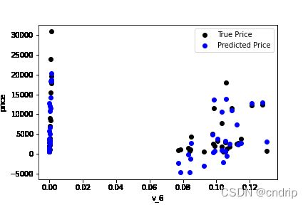
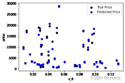
分别对v_6、v_8 和 v_9 进行可视化
from matplotlib import pyplot as plt
subsample_index = np.random.randint(low=0, high=len(train_y), size=50)
plt.scatter(train_X['v_9'][subsample_index], train_y[subsample_index], color='black')
plt.scatter(train_X['v_9'][subsample_index], model.predict(train_X.loc[subsample_index]), color='blue')
plt.xlabel('v_9')
plt.ylabel('price')
plt.legend(['True Price','Predicted Price'],loc='upper right')
print('The predicted price is obvious different from true price')
plt.show()
绘制特征v_9的值与标签的散点图,图片发现模型的预测结果(蓝色点)与真实标签(黑色点)的分布差异较大,且部分预测值出现了小于0的情况,说明我们的模型存在一些问题。
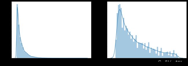
通过作图我们发现数据的标签(price)呈现长尾分布,不利于我们的建模预测。原因是很多模型都假设数据误差项符合正态分布,而长尾分布的数据违背了这一假设。
import seaborn as sns
print('It is clear to see the price shows a typical exponential distribution')
plt.figure(figsize=(15,5))
plt.subplot(1,2,1)
sns.distplot(train_y)
plt.subplot(1,2,2)
sns.distplot(train_y[train_y < np.quantile(train_y, 0.9)])
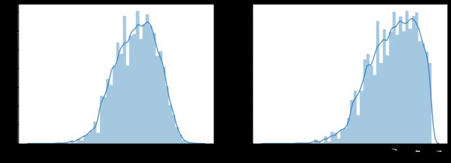
在这里我们对标签进行了 l o g ( x + 1 ) log(x+1) log(x+1) 变换,使标签贴近于正态分布
train_y_ln = np.log(train_y + 1)
import seaborn as sns
print('The transformed price seems like normal distribution')
plt.figure(figsize=(15,5))
plt.subplot(1,2,1)
sns.distplot(train_y_ln)
plt.subplot(1,2,2)
sns.distplot(train_y_ln[train_y_ln < np.quantile(train_y_ln, 0.9)])
处理后重新建模
model = model.fit(train_X, train_y_ln)

print('intercept:'+ str(model.intercept_))
sorted(dict(zip(continuous_feature_names, model.coef_)).items(), key=lambda x:x[1], reverse=True)
'''
以下是部分结果
intercept:18.75074572712829
[('v_9', 8.052411938253034),
, ('v_5', 5.76424821734175),
, ('v_12', 1.6182065931157121),
, ('v_1', 1.479830409604984),
'''
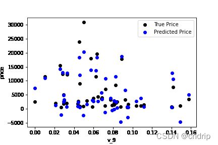
再次进行可视化,发现预测结果与真实值较为接近,且未出现异常状况
plt.scatter(train_X['v_9'][subsample_index], train_y[subsample_index], color='black')
plt.scatter(train_X['v_9'][subsample_index], np.exp(model.predict(train_X.loc[subsample_index])), color='blue')
plt.xlabel('v_9')
plt.ylabel('price')
plt.legend(['True Price','Predicted Price'],loc='upper right')
print('The predicted price seems normal after np.log transforming')
plt.show()
2.2 五折交叉验证
在使用训练集对参数进行训练的时候,经常会发现人们通常会将一整个训练集分为三个部分(比如mnist手写训练集)。一般分为:训练集(train_set),评估集(valid_set),测试集(test_set)这三个部分。这其实是为了保证训练效果而特意设置的。其中测试集很好理解,其实就是完全不参与训练的数据,仅仅用来观测测试效果的数据。而训练集和评估集则牵涉到下面的知识了。
因为在实际的训练中,训练的结果对于训练集的拟合程度通常还是挺好的(初始条件敏感),但是对于训练集之外的数据的拟合程度通常就不那么令人满意了。因此我们通常并不会把所有的数据集都拿来训练,而是分出一部分来(这一部分不参加训练)对训练集生成的参数进行测试,相对客观的判断这些参数对训练集之外的数据的符合程度。这种思想就称为交叉验证(Cross Validation)
from sklearn.model_selection import cross_val_score
from sklearn.metrics import mean_absolute_error,  make_scorer
def log_transfer(func):
    def wrapper(y, yhat):
        result = func(np.log(y), np.nan_to_num(np.log(yhat)))
        return result
    return wrapper
scores = cross_val_score(model, X=train_X, y=train_y, verbose=1, cv = 5, scoring=make_scorer(log_transfer(mean_absolute_error)))
[Parallel(n_jobs=1)]: Done 5 out of 5 | elapsed: 6.5s finished
使用线性回归模型,对未处理标签的特征数据进行五折交叉验证
print('AVG:', np.mean(scores))
# AVG: 1.3658024040276566
使用线性回归模型,对处理过标签的特征数据进行五折交叉验证
scores = cross_val_score(model, X=train_X, y=train_y_ln, verbose=1, cv = 5, scoring=make_scorer(mean_absolute_error))
[Parallel(n_jobs=1)]: Done 5 out of 5 | elapsed: 8.4s finished
print('AVG:', np.mean(scores))
# AVG: 0.1932530155796405
scores = pd.DataFrame(scores.reshape(1,-1))
scores.columns = ['cv' + str(x) for x in range(1, 6)]
scores.index = ['MAE']
scores
| cv1 | cv2 | cv3 | cv4 | cv5 | |
|---|---|---|---|---|---|
| MAE | 0.190792 | 0.193758 | 0.194132 | 0.191825 | 0.195758 |
2.3 模拟真实业务情况
但在事实上,由于我们并不具有预知未来的能力,五折交叉验证在某些与时间相关的数据集上反而反映了不真实的情况。通过2018年的二手车价格预测2017年的二手车价格,这显然是不合理的,因此我们还可以采用时间顺序对数据集进行分隔。在本例中,我们选用靠前时间的4/5样本当作训练集,靠后时间的1/5当作验证集,最终结果与五折交叉验证差距不大
import datetime
sample_feature = sample_feature.reset_index(drop=True)
split_point = len(sample_feature) // 5 * 4
train = sample_feature.loc[:split_point].dropna()
val = sample_feature.loc[split_point:].dropna()

train_X = train[continuous_feature_names]
train_y_ln = np.log(train['price'] + 1)
val_X = val[continuous_feature_names]
val_y_ln = np.log(val['price'] + 1)
model = model.fit(train_X, train_y_ln)
mean_absolute_error(val_y_ln, model.predict(val_X))
0.19577667149549252
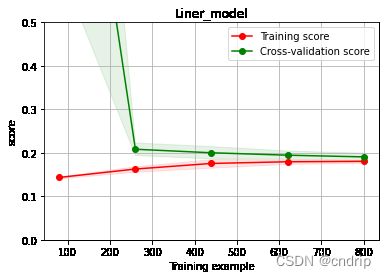
2.4 绘制学习率曲线与验证曲线
from sklearn.model_selection import learning_curve, validation_curve
# ? learning_curve 通过问号,查看使用指南
def plot_learning_curve(estimator, title, X, y, ylim=None, cv=None,n_jobs=1, train_size=np.linspace(.1, 1.0, 5 )):
    plt.figure()
    plt.title(title)
    if ylim is not None:
        plt.ylim(*ylim)
    plt.xlabel('Training example')
    plt.ylabel('score')
    train_sizes, train_scores, test_scores = learning_curve(estimator, X, y, cv=cv, n_jobs=n_jobs, train_sizes=train_size, scoring = make_scorer(mean_absolute_error))
    train_scores_mean = np.mean(train_scores, axis=1)
    train_scores_std = np.std(train_scores, axis=1)
    test_scores_mean = np.mean(test_scores, axis=1)
    test_scores_std = np.std(test_scores, axis=1)
    plt.grid()#区域
    plt.fill_between(train_sizes, train_scores_mean - train_scores_std,
                     train_scores_mean + train_scores_std, alpha=0.1,
                     color="r")
    plt.fill_between(train_sizes, test_scores_mean - test_scores_std,
                     test_scores_mean + test_scores_std, alpha=0.1,
                     color="g")
    plt.plot(train_sizes, train_scores_mean, 'o-', color='r',
             label="Training score")
    plt.plot(train_sizes, test_scores_mean,'o-',color="g",
             label="Cross-validation score")
    plt.legend(loc="best")
    return plt
plot_learning_curve(LinearRegression(), 'Liner_model', train_X[:1000], train_y_ln[:1000], ylim=(0.0, 0.5), cv=5, n_jobs=1)
3 多种模型对比
train = sample_feature[continuous_feature_names + ['price']].dropna()

train_X = train[continuous_feature_names]
train_y = train['price']
train_y_ln = np.log(train_y + 1)
3.1 线性模型 & 嵌入式特征选择
本章节默认,学习者已经了解关于过拟合、模型复杂度、正则化等概念。否则请寻找相关资料或参考如下连接:
 - 用简单易懂的语言描述「过拟合 overfitting」? https://www.zhihu.com/question/32246256/answer/55320482
 - 模型复杂度与模型的泛化能力 http://yangyingming.com/article/434/
 - 正则化的直观理解 https://blog.csdn.net/jinping_shi/article/details/52433975
在过滤式和包裹式特征选择方法中,特征选择过程与学习器训练过程有明显的分别。而嵌入式特征选择在学习器训练过程中自动地进行特征选择。嵌入式选择最常用的是L1正则化与L2正则化。在对线性回归模型加入两种正则化方法后,他们分别变成了岭回归与Lasso回归。
from sklearn.linear_model import LinearRegression
from sklearn.linear_model import Ridge
from sklearn.linear_model import Lasso
models = [LinearRegression(),
          Ridge(),
          Lasso()]
result = dict()
for model in models:
    model_name = str(model).split('(')[0]
    scores = cross_val_score(model, X=train_X, y=train_y_ln, verbose=0, cv = 5, scoring=make_scorer(mean_absolute_error))
    result[model_name] = scores
    print(model_name + ' is finished')
运行后,对三种方法的效果对比
result = pd.DataFrame(result)
result.index = ['cv' + str(x) for x in range(1, 6)]
result
'''
	LinearRegression	Ridge	Lasso
cv1	0.190792	0.194832	0.383899
cv2	0.193758	0.197632	0.381893
cv3	0.194132	0.198123	0.384090
cv4	0.191825	0.195670	0.380526
cv5	0.195758	0.199676	0.383611
'''
model = LinearRegression().fit(train_X, train_y_ln)
print('intercept:'+ str(model.intercept_))
# intercept:18.750751045631276
sns.barplot(abs(model.coef_), continuous_feature_names)
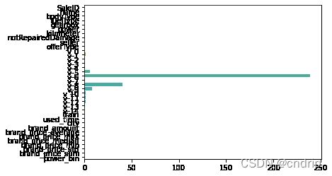
L2正则化在拟合过程中通常都倾向于让权值尽可能小,最后构造一个所有参数都比较小的模型。因为一般认为参数值小的模型比较简单,能适应不同的数据集,也在一定程度上避免了过拟合现象。可以设想一下对于一个线性回归方程,若参数很大,那么只要数据偏移一点点,就会对结果造成很大的影响;但如果参数足够小,数据偏移得多一点也不会对结果造成什么影响,专业一点的说法是『抗扰动能力强』
model = Ridge().fit(train_X, train_y_ln)
print('intercept:'+ str(model.intercept_))
# intercept:4.671710811023084
sns.barplot(abs(model.coef_), continuous_feature_names)
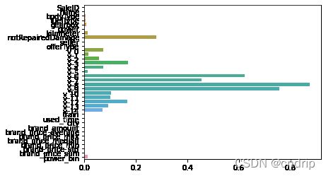
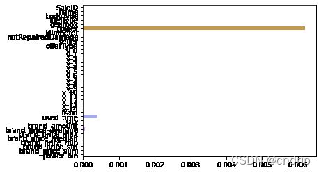
L1正则化有助于生成一个稀疏权值矩阵,进而可以用于特征选择。如下图,我们发现power与userd_time特征非常重要。
model = Lasso().fit(train_X, train_y_ln)
print('intercept:'+ str(model.intercept_))
# intercept:8.67218477236799
sns.barplot(abs(model.coef_), continuous_feature_names)
除此之外,决策树通过信息熵或GINI指数选择分裂节点时,优先选择的分裂特征也更加重要,这同样是一种特征选择的方法。XGBoost与LightGBM模型中的model_importance指标正是基于此计算的
3.2 非线性模型
from sklearn.linear_model import LinearRegression
from sklearn.svm import SVC
from sklearn.tree import DecisionTreeRegressor
from sklearn.ensemble import RandomForestRegressor
from sklearn.ensemble import GradientBoostingRegressor
from sklearn.neural_network import MLPRegressor
from xgboost.sklearn import XGBRegressor
from lightgbm.sklearn import LGBMRegressor
models = [LinearRegression(),
          DecisionTreeRegressor(),
          RandomForestRegressor(),
          GradientBoostingRegressor(),
          MLPRegressor(solver='lbfgs', max_iter=100),
          XGBRegressor(n_estimators = 100, objective='reg:squarederror'),
          LGBMRegressor(n_estimators = 100)]
以下代码运行不少时间(近30分钟)
result = dict()
for model in models:
    model_name = str(model).split('(')[0]
    scores = cross_val_score(model, X=train_X, y=train_y_ln, verbose=0, cv = 5, scoring=make_scorer(mean_absolute_error))
    result[model_name] = scores
    print(model_name + ' is finished')
result = pd.DataFrame(result)
result.index = ['cv' + str(x) for x in range(1, 6)]
result
| LinearRegression | DecisionTreeRegressor | RandomForestRegressor | GradientBoostingRegressor | MLPRegressor | XGBRegressor | LGBMRegressor | |
|---|---|---|---|---|---|---|---|
| cv1 | 0.190792 | 0.197389 | 0.141478 | 0.168897 | 1001.733766 | 0.169990 | 0.141544 |
| cv2 | 0.193758 | 0.191933 | 0.143521 | 0.171852 | 417.772333 | 0.171826 | 0.145501 |
| cv3 | 0.194132 | 0.189844 | 0.141509 | 0.170875 | 966.174349 | 0.172123 | 0.143887 |
| cv4 | 0.191825 | 0.189257 | 0.140547 | 0.169064 | 848.035829 | 0.169635 | 0.142497 |
| cv5 | 0.195758 | 0.204853 | 0.146956 | 0.174094 | 637.565235 | 0.172824 | 0.144852 |
可以看到随机森林模型在每一个fold中均取得了更好的效果
4 模型调参
在此我们介绍了三种常用的调参方法如下:
- 贪心算法 https://www.jianshu.com/p/ab89df9759c8
- 网格调参 https://blog.csdn.net/weixin_43172660/article/details/83032029
- 贝叶斯调参 https://blog.csdn.net/linxid/article/details/81189154
## LGB的参数集合:

objective = ['regression', 'regression_l1', 'mape', 'huber', 'fair']

num_leaves = [3,5,10,15,20,40, 55]
max_depth = [3,5,10,15,20,40, 55]
bagging_fraction = []
feature_fraction = []
drop_rate = []
4.1 贪心调参
best_obj = dict()
for obj in objective:
    model = LGBMRegressor(objective=obj)
    score = np.mean(cross_val_score(model, X=train_X, y=train_y_ln, verbose=0, cv = 5, scoring=make_scorer(mean_absolute_error)))
    best_obj[obj] = score

best_leaves = dict()
for leaves in num_leaves:
    model = LGBMRegressor(objective=min(best_obj.items(), key=lambda x:x[1])[0], num_leaves=leaves)
    score = np.mean(cross_val_score(model, X=train_X, y=train_y_ln, verbose=0, cv = 5, scoring=make_scorer(mean_absolute_error)))
    best_leaves[leaves] = score

best_depth = dict()
for depth in max_depth:
    model = LGBMRegressor(objective=min(best_obj.items(), key=lambda x:x[1])[0],
                          num_leaves=min(best_leaves.items(), key=lambda x:x[1])[0],
                          max_depth=depth)
    score = np.mean(cross_val_score(model, X=train_X, y=train_y_ln, verbose=0, cv = 5, scoring=make_scorer(mean_absolute_error)))
    best_depth[depth] = score
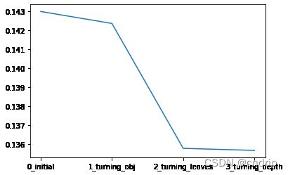
以下代码运行需近10分钟
sns.lineplot(x=['0_initial','1_turning_obj','2_turning_leaves','3_turning_depth'], y=[0.143 ,min(best_obj.values()), min(best_leaves.values()), min(best_depth.values())])
4.2 Grid Search 调参
from sklearn.model_selection import GridSearchCV
parameters = {'objective': objective , 'num_leaves': num_leaves, 'max_depth': max_depth}
model = LGBMRegressor()
clf = GridSearchCV(model, parameters, cv=5)
clf = clf.fit(train_X, train_y)
clf.best_params_
{‘max_depth’: 15, ‘num_leaves’: 55, ‘objective’: ‘regression’}
model = LGBMRegressor(objective='regression',
                          num_leaves=55,
                          max_depth=15)
np.mean(cross_val_score(model, X=train_X, y=train_y_ln, verbose=0, cv = 5, scoring=make_scorer(mean_absolute_error)))
#0.1375483296069761
4.3 贝叶斯调参
from bayes_opt import BayesianOptimization
def rf_cv(num_leaves, max_depth, subsample, min_child_samples):
    val = cross_val_score(
        LGBMRegressor(objective = 'regression_l1',
            num_leaves=int(num_leaves),
            max_depth=int(max_depth),
            subsample = subsample,
            min_child_samples = int(min_child_samples)
        ),
        X=train_X, y=train_y_ln, verbose=0, cv = 5, scoring=make_scorer(mean_absolute_error)
    ).mean()
    return 1 - val
rf_bo = BayesianOptimization(
rf_cv,
{
'num_leaves': (2, 100),
'max_depth': (2, 100),
'subsample': (0.1, 1),
'min_child_samples' : (2, 100)
}
)
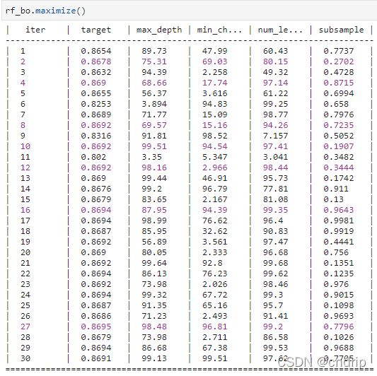
rf_bo.maximize()
'''
| iter | target | max_depth | min_ch... | num_le... | subsample |
-------------------------------------------------------------------------
| 1 | 0.8654 | 89.73 | 47.99 | 60.43 | 0.7737 |
| 2 | 0.8678 | 75.31 | 69.03 | 80.15 | 0.2702 |
| 3 | 0.8632 | 94.39 | 2.258 | 49.32 | 0.4728 |
| 4 | 0.869 | 68.66 | 17.74 | 97.14 | 0.8715 |
| 5 | 0.8655 | 56.37 | 3.616 | 61.22 | 0.6994 |
| 6 | 0.8253 | 3.894 | 94.83 | 99.25 | 0.658 |
| 7 | 0.8689 | 71.77 | 15.09 | 98.77 | 0.7976 |
| 8 | 0.8692 | 69.57 | 15.16 | 94.26 | 0.7235 |
| 9 | 0.8316 | 91.81 | 98.52 | 7.157 | 0.5052 |
| 10 | 0.8692 | 99.51 | 94.54 | 97.41 | 0.1907 |
| 11 | 0.802 | 3.35 | 5.347 | 3.041 | 0.3482 |
| 12 | 0.8692 | 98.16 | 2.966 | 98.44 | 0.3444 |
| 13 | 0.869 | 99.44 | 46.91 | 95.73 | 0.1742 |
| 14 | 0.8676 | 99.2 | 96.79 | 77.81 | 0.911 |
| 15 | 0.8679 | 83.65 | 2.167 | 81.08 | 0.13 |
| 16 | 0.8694 | 87.95 | 94.39 | 99.35 | 0.9643 |
| 17 | 0.8694 | 98.99 | 76.62 | 96.4 | 0.9981 |
| 18 | 0.8687 | 85.95 | 32.62 | 90.83 | 0.9919 |
| 19 | 0.8692 | 56.89 | 3.561 | 97.47 | 0.4441 |
| 20 | 0.869 | 80.05 | 2.333 | 96.68 | 0.756 |
| 21 | 0.8692 | 99.64 | 92.8 | 99.68 | 0.1351 |
| 22 | 0.8694 | 86.13 | 76.23 | 99.62 | 0.1235 |
| 23 | 0.8692 | 73.98 | 2.026 | 98.46 | 0.976 |
| 24 | 0.8694 | 99.32 | 67.72 | 99.3 | 0.9015 |
| 25 | 0.8687 | 91.35 | 65.16 | 95.7 | 0.1098 |
| 26 | 0.8686 | 71.23 | 2.493 | 91.41 | 0.9693 |
| 27 | 0.8695 | 98.48 | 96.81 | 99.2 | 0.7796 |
| 28 | 0.8679 | 73.98 | 2.711 | 86.58 | 0.1026 |
| 29 | 0.8694 | 86.68 | 67.38 | 99.53 | 0.9688 |
| 30 | 0.8691 | 99.13 | 99.51 | 97.62 | 0.7705 |
=========================================================================
'''
1 - rf_bo.max['target']
# 0.13051612046516825
# 第27号为最优参数
以下代码和图引自 小雨姑娘
plt.figure(figsize=(13,5))
sns.lineplot(x=['0_origin','1_log_transfer','2_L1_&_L2','3_change_model','4_parameter_turning'], y=[1.36 ,0.19, 0.19, 0.14, 0.13])

学习问题与解答
问题1 :简单建模后需要可视化所有特征吗
- 解答:先查看前3-5个权重的特征,可视频化后,查看预测值与真实值是否接近,是否出现异常情况,如出现负值等
问题2 : 调参神器贝叶斯优化(bayesian-optimization)
- 解答:
- 原理:利用已有的先验信息去找到使目标函数达到全局最大的参数。
- 贝叶斯调参相对于网格搜索的优势:
- 贝叶斯调参采用高斯过程,会考虑到之前的参数信息,不断地更新先验;网格搜索则不会考虑先验信息。
- 贝叶斯调参迭代次数少,速度快;网格搜索会遍历所有的可能的参数组合,所以速度慢,参数多时易导致维度爆炸
- 贝叶斯调参针对非凸问题依然稳健;网格搜索针对非凸问题易得到局部最优。
- 一旦出现更好的参数空间,会有通过不同颜色来区别。
学习思考与总结
通过各模型的比较,首先对各种模型的复杂度要有一个总体的了解,一般先复杂度低的模型,因为在调参过程是非常耗时间,较复杂的模型跑一次就得花10-20分钟时间,所以在调参过程,需要考虑时间成本,以及效率。
如果为了比赛,提高 0.01 ,多花30分种,那也是可以的。
贝叶斯调参是一种值得推荐的方法,充分利用已有的先验信息去找到使目标函数达到全局最大的参数,是一种逐步求精的方法。