Simulation | Multi-Armed Bandit Algorithm
Simulation | Multi-Armed Bandit Algorithm
I. Propose
∙ \bullet ∙ Simulation of Multi-Armed Bandit Algorithms: ε \varepsilon ε-Greedy, UCB(Upper Confidence Bound), Thompson Sampling and Gradient Bandit Algorithm.
∙ \bullet ∙ Compare the algorithms with different parameter and give explanation for these impact.
∙ \bullet ∙ Explain the understanding of the exploration-exploitation trade-off in bandit-algorithms.
∙ \bullet ∙ Solve the further problem: dependent case.
∙ \bullet ∙ Explain why sublinear regret is the performance threshold between good bandit algorithms and bad one.
II. Simulation
Step 1: Oracle Value of Bernoulli Distribution
Suppose we have known the true values of the parameters of the Bernoulli Distribution B e r n ( θ j ) Bern( \theta_j ) Bern(θj) of each arm (the probability of each bandit gives a reward) as below:
θ 1 = 0.9 , θ 2 = 0.8 , θ 3 = 0.7 \theta_1 = 0.9,\theta_2 = 0.8,\theta_3 = 0.7 θ1=0.9,θ2=0.8,θ3=0.7
We can use the parameters above to compute the expectation of aggregate rewards of each arm over N=10000 times slots, which can be achieved by testing Bin( N N N, θ j \theta_j θj) .
The test function with parameters θ j \theta_j θj is as below:
import math
import random
import numpy as np
from collections import Counter
import matplotlib.pyplot as plt
from scipy.stats import beta

def oracle(N,theta):
    # experiments of bin(n, theta)
    arm = np.random.binomial(1,theta,N)

    #output the total times of success
    return Counter(arm)[1]
The test function above outputs the total successful times of Bern( θ j \theta_j θj) over N N N times slots. Then we can use the function to compute the theoretically maximized expected rewards (oracle value).
The result is as below:
def Oracle(arm_mean,N):

    #first arm with theta_1 = 0.8
    arm_1 = oracle(N,arm_mean[0])

    #second bandit with theta_2 = 0.6
    arm_2 = oracle(N,arm_mean[1])

    #third bandit with theta_3 = 0.5
    arm_3 = oracle(N,arm_mean[2])

    #compute the maximum of the expectation of three bandits
    arm = np.array([arm_1,arm_2,arm_3])
    max_i = np.argmax(arm)
    maximum = max(arm_1,arm_2,arm_3)

    return maximum,max_i

arm_mean = [0.9,0.8,0.7]
N = 10000

oracle_value,max_i = Oracle(arm_mean,N)
print("The oracle value is {}, from arm {}.".format(oracle_value,max_i+1))
![]()
From the result, we can find if we have known the probability of success of each arm: θ j \theta_j θj, it is obvious to choose the bandit with the maximized probability to get the theoretically maximized aggregate expectation, which is the oracle value.
To test the performance of these algorithms, firstly we generate a function named run_algorithm to run these three algorithm. The final ouput is arrays that record the mean of average reward and cumlative reward after each experiment with N = 5000 N=5000 N=5000 slots.
def run_algorithm(algo, arms, num_exper, num_slot):

    #initialize the arrays record the rewards and chosen arms
    rewards = np.zeros((num_exper,num_slot))
    chosen_arm = np.zeros((num_exper,num_slot))

    for exper in range(num_exper):

        #initialize the algorithm
        algo.initialize(len(arms))

        for slot in range(num_slot):

            #obtain the factor of update
            arm = algo.best_arm()
            reward = arms[arm].draw()

            #update the data
            chosen_arm[exper,slot] = arm
            rewards[exper,slot] = reward
            algo.update(arm,reward,slot)

    #compute the average and cumulation of rewards
    average_reward = np.mean(rewards,axis=0)
    cumulative_reward = np.cumsum(average_reward)

    return chosen_arm,average_reward,cumulative_reward
Also, we need to generate a function named plot_algorithm to plot the output of each algorithm. And then we can compare the performance of each algorithm with different parameters by the plots.
def plot_algorithm(algo_name, para, arms, arm_mean, num_exper, num_slot, label):

    fig,axes = plt.subplots(2,2,figsize=[15,9])
    R = []
    Percentage = []
    optimal_arm = np.argmax(arm_mean)

    #Greedy and UCB
    if algo_name == Greedy or algo_name == UCB:
        for para in para:

            #run the algorithm
            algo = algo_name(para)
            chosen_arm,average_reward,cumulative_reward = \
                run_algorithm(algo,arms,num_exper,num_slot)

            #plot the average reward
            axes[0][0].plot(average_reward,label=f"{label} = {para}")
            axes[0][0].set_xlabel("Slots")
            axes[0][0].set_ylabel("Average Reward")
            axes[0][0].set_title("Average Reward")
            axes[0][0].legend(loc="lower right")
            axes[0][0].set_ylim([0, 1.0])

            #plot the cumulative reward
            axes[0][1].plot(cumulative_reward,label=f"{label} = {para}")
            axes[0][1].set_xlabel("Slots")
            axes[0][1].set_ylabel("Cumulative Reward")
            axes[0][1].set_title("Cumulative Reward")
            axes[0][1].legend(loc="lower right")

            #regret part
            regret = np.zeros((num_exper,num_slot))
            average_regret = np.zeros(num_slot)
            optimal_num = np.zeros(num_slot)
            optimal_percent = np.zeros(num_slot)

            #calculate the regret
            for exper in range(num_exper):
                for slot in range(num_slot):
                    regret[exper,slot] = arm_mean[optimal_arm] - arm_mean[int(chosen_arm[exper,slot])]
                    if int(chosen_arm[exper,slot]) == optimal_arm:
                        optimal_num[slot] += 1
            optimal_percent = optimal_num/num_exper
            average_percent = np.mean(optimal_percent)
            average_regret = np.mean(regret,axis=0)
            total_regret = np.sum(average_regret)
            cumulative_regret = np.cumsum(average_regret)

            #plot the regret as a function of time
            axes[1][0].plot(cumulative_regret,label=f"{label} = {para}")
            axes[1][0].set_xlabel("Slots")
            axes[1][0].set_ylabel("Cumulative Regret")
            axes[1][0].set_title("Cumulative Regret")
            axes[1][0].legend(loc="lower right")

            #plot the optimal action percent as a function of slots
            axes[1][1].plot(optimal_percent,label=f"{label} = {para}")
            axes[1][1].set_xlabel("Slots")
            axes[1][1].set_ylabel("Percent")
            axes[1][1].set_title("Optimal action Selection")
            axes[1][1].legend(loc="lower right")
            axes[1][1].set_ylim([0, 1.0])

            #print the total regret accumulated over each experiment
            print("{} = {}: The total regret accumulated is {:.4f}.".format(label,para,total_regret))

            #print the average percentage of plays in which the optimal arm is pulled
            print("{} = {}: The average percentage of optimal arm is pulled is {:.4f}.".format(label,para,average_percent))

            reward = cumulative_reward[num_slot-1]
            R.append(reward)
            Percentage.append(average_percent)

    #Thompson Sampling
    elif algo_name == TS:
        i = 1
        for para in para:

            #run the algorithm
            algo = algo_name(para[0],para[1])
            chosen_arm,average_reward,cumulative_reward = \
                run_algorithm(algo,arms,num_exper,num_slot)

            #plot the average reward
            axes[0][0].plot(average_reward,label="beta"+str(i))
            axes[0][0].set_xlabel("Slots")
            axes[0][0].set_ylabel("Average Reward")
            axes[0][0].set_title("Average Reward")
            axes[0][0].legend(loc="lower right")
            axes[0][0].set_ylim([0, 1.0])

            #plot the cumulative reward
            axes[0][1].plot(cumulative_reward,label="beta"+str(i))
            axes[0][1].set_xlabel("Slots")
            axes[0][1].set_ylabel("Cumulative Reward")
            axes[0][1].set_title("Cumulative Reward")
            axes[0][1].legend(loc="lower right")

            #regret part
            regret = np.zeros((num_exper,num_slot))
            average_regret = np.zeros(num_slot)
            optimal_num = np.zeros(num_slot)
            optimal_percent = np.zeros(num_slot)

            #calculate the regret
            for exper in range(num_exper):
                for slot in range(num_slot):
                    regret[exper,slot] = arm_mean[optimal_arm] - arm_mean[int(chosen_arm[exper,slot])]
                    if int(chosen_arm[exper,slot]) == optimal_arm:
                        optimal_num[slot] += 1
            optimal_percent = optimal_num/num_exper
            average_percent = np.mean(optimal_percent)
            average_regret = np.mean(regret,axis=0)
            total_regret = np.sum(average_regret)
            cumulative_regret = np.cumsum(average_regret)

            #plot the regret as a function of time
            axes[1][0].plot(cumulative_regret,label="beta"+str(i))
            axes[1][0].set_xlabel("Slots")
            axes[1][0].set_ylabel("Cumulative Regret")
            axes[1][0].set_title("Cumulative Regret")
            axes[1][0].legend(loc="lower right")

            #plot the optimal action percent as a function of slots
            axes[1][1].plot(optimal_percent,label="beta"+str(i))
            axes[1][1].set_xlabel("Slots")
            axes[1][1].set_ylabel("Percent")
            axes[1][1].set_title("Optimal action Selection")
            axes[1][1].legend(loc="lower right")
            axes[1][1].set_ylim([0, 1.0])

            #print the total regret accumulated over each experiment
            print("beta{}: The total regret accumulated over the experiment is {:.4f}.".format(str(i),total_regret))

            #print the average percentage of plays in which the optimal arm is pulled
            print("beta{}: The average percentage of optimal arm is pulled is {:.4f}.".format(str(i),average_percent))

            i += 1
            reward = cumulative_reward[num_slot-1]
            R.append(reward)
            Percentage.append(average_percent)

    #Gradient bandit
    elif algo_name == Gradient:
        i = 1
        for para in para:

            #run the algorithm
            algo = algo_name(step_size = para[0], baseline = para[1], beta = para[2])
            chosen_arm,average_reward,cumulative_reward = \
                run_algorithm(algo,arms,num_exper,num_slot)

            #plot the average reward
            axes[0][0].plot(average_reward,label=f"{label} = {para}")
            axes[0][0].set_xlabel("Slots")
            axes[0][0].set_ylabel("Average Reward")
            axes[0][0].set_title("Average Reward")
            axes[0][0].legend(loc="lower right")
            axes[0][0].set_ylim([0, 1.0])

            #plot the cumulative reward
            axes[0][1].plot(cumulative_reward,label=f"{label} = {para}")
            axes[0][1].set_xlabel("Slots")
            axes[0][1].set_ylabel("Cumulative Reward")
            axes[0][1].set_title("Cumulative Reward")
            axes[0][1].legend(loc="lower right")

            #regret part
            regret = np.zeros((num_exper,num_slot))
            average_regret = np.zeros(num_slot)
            optimal_num = np.zeros(num_slot)
            optimal_percent = np.zeros(num_slot)

            #calculate the regret
            for exper in range(num_exper):
                for slot in range(num_slot):
                    regret[exper,slot] = arm_mean[optimal_arm] - arm_mean[int(chosen_arm[exper,slot])]
                    if int(chosen_arm[exper,slot]) == optimal_arm:
                        optimal_num[slot] += 1
            optimal_percent = optimal_num/num_exper
            average_percent = np.mean(optimal_percent)
            average_regret = np.mean(regret,axis=0)
            total_regret = np.sum(average_regret)
            cumulative_regret = np.cumsum(average_regret)

            #plot the regret as a function of time
            axes[1][0].plot(cumulative_regret,label=f"{label} = {para}")
            axes[1][0].set_xlabel("Slots")
            axes[1][0].set_ylabel("Cumulative Regret")
            axes[1][0].set_title("Cumulative Regret")
            axes[1][0].legend(loc="lower right")

            #plot the optimal action percent as a function of slots
            axes[1][1].plot(optimal_percent,label=f"{label} = {para}")
            axes[1][1].set_xlabel("Slots")
            axes[1][1].set_ylabel("Percent")
            axes[1][1].set_title("Optimal action Selection")
            axes[1][1].legend(loc="lower right")
            axes[1][1].set_ylim([0, 1.0])

            #print the total regret accumulated over each experiment
            print("para{}: The total regret accumulated over the experiment is {:.4f}.".format(str(i),total_regret))

            #print the average percentage of plays in which the optimal arm is pulled
            print("para{}: The average percentage of optimal arm is pulled is {:.4f}.".format(str(i),average_percent))

            i += 1
            reward = cumulative_reward[num_slot-1]
            R.append(reward)
            Percentage.append(average_percent)

    plt.subplots_adjust(hspace=0.3)
    plt.show()

    print("The best arm is Arm{} with mean = {}"\
        .format(optimal_arm+1,arm_mean[optimal_arm]))
    return max(R), np.argmax(R), average_percent, max(Percentage)
Step 2: Implementing bandit algorithms
Firstly we need to create a class named “Bern_arm” to represent the arms of bandit. This class enables us to obtain a random reward based on the mean of each arm.
class Bern_arm:
    def __init__(self, mean):
        self.mean = mean

    def draw(self):
        i = np.random.uniform(0,1)

        if i < self.mean:
            return 1
        else:
            return 0
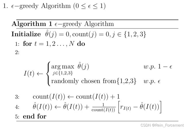
1. ε \varepsilon ε-Greedy Algorithm
ε \varepsilon ε-Greedy Algorithm can be defined as the algorithm to choose the arm which has the largest mean before and have a probability to randomly choose other arm, by which we can achieve both the exploition strategy (probability = 1 − ε 1-\varepsilon 1−ε) and exploration strategy (probability = ε \varepsilon ε) randomly.
The class “Greedy” is to generate a algorithm class to achieve ε \varepsilon ε-Greedy Algorithm. It has three basic process: initialization, choosing the best arm, updating mean reward.
class Greedy:
    def __init__(self, epsilon, count = None, mean = None):
        self.epsilon = epsilon
        self.count = count
        self.mean = mean

    def initialize(self, num_arms):
        self.count = np.zeros(num_arms)
        self.mean = np.zeros(num_arms)

    def best_arm(self):
        i = random.uniform(0,1)

        if i < self.epsilon:
            #random choose the arms
            return np.random.randint(0,len(self.mean)-1)

        else:
            #choose the arm with the maximum mean
            return np.argmax(self.mean)

    def update(self, chosen_arm, reward, slot):

        #update the count of the chosen arm by one
        self.count[chosen_arm] += 1

        #update the estimated mean of the chosen arm
        self.mean[chosen_arm] += (reward-self.mean[chosen_arm])/ \
                                    self.count[chosen_arm]
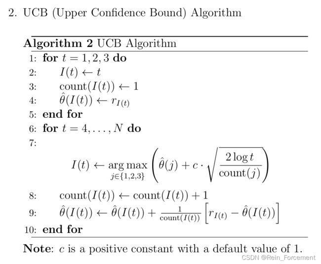
2. UCB Algorithm
Upper Confidence Bounds(UCB) Algorithm measures the exploration of actions with a strong potential to have a optimal value by an upper confidence bound of the reward value.
The class “UCB” is to generate a algorithm class to achieve UCB Algorithm. It has the similar process with the previous one.
class UCB:
    def __init__(self, c, count = None, mean = None):
        self.count = count
        self.mean = mean
        self.c = c

    def initialize(self, num_arms):
        self.count = np.zeros(num_arms)
        self.mean = np.zeros(num_arms)
        self.num_arms = num_arms
        self.t = 0

    def best_arm(self):

        if self.t <= self.num_arms-1:
            return self.t

        else:
            #choose the best arm
            return np.argmax(self.mean + \
                self.c*math.sqrt(2*math.log(self.t))/self.count)

    def update(self, chosen_arm, reward, slot):

        if self.t <= self.num_arms-1:
            self.count[self.t] = 1
            self.mean[self.t] = reward

        else:
            #update the count of the chosen arm by one
            self.count[chosen_arm] += 1

            #update the estimated mean of the chosen arm
            self.mean[chosen_arm] += (reward-self.mean[chosen_arm])/ \
                                        self.count[chosen_arm]

        self.t += 1
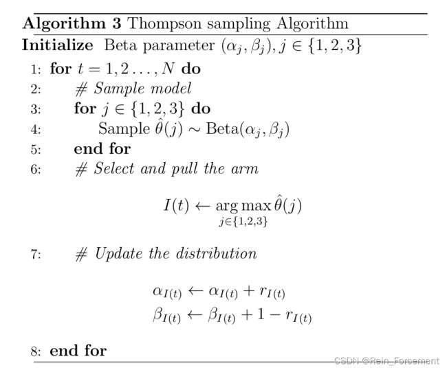
3. Thompson Sampling (TS) Algorithm
Thompson Sampling is an algorithm for online decision problems where actions are taken sequentially in a manner that must balance between exploiting what is known to maximize immediate performance and investing to accumulate new information that may improve future performance. The algorithm addresses a broad range of problems in a computationally efficient manner and is therefore enjoying wide use.
The class “TS” is to generate a algorithm class to achieve Thompson Sampling Algorithm. It has the similar process with the previous two.
class TS:
    def __init__(self, alpha, beta, mean = None):
        self.alpha = alpha
        self.beta = beta
        self.mean = mean

    def initialize(self, num_arms):
        self.num_arms = num_arms
        self.mean = np.zeros(num_arms)

    def best_arm(self):
        for i in range(self.num_arms):
            self.mean[i] = np.random.beta(self.alpha[i],self.beta[i])

        #choose the arm with the maximum mean
        return np.argmax(self.mean)

    def update(self, chosen_arm, reward, slot):

        #update the parameter alpha and beta
        self.alpha[chosen_arm] += reward
        self.beta[chosen_arm] += 1-reward
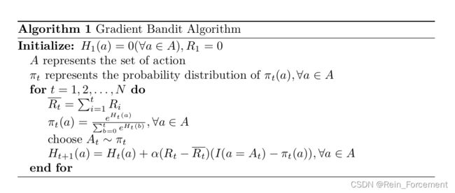
4. (Parameterized) Gradient Bandit Algorithm
# time-varying parameter beta: beta = log(t)
def Beta(slot):
    if slot != 0:
        return math.log(slot)
    else:
        return 0

class Gradient:
    def __init__(self, step_size = 0.1, baseline = None, beta = None):
        if step_size == None:
            self.lr = 0.1
        else:
            self.lr = step_size
        # beta not equal to none means beta is a constant.
        # Otherwise, it is a time-varing function
        if beta != None:
            self.beta = beta

        # if there is no value of baseline is passed in,
        # then we set the baseline to be the average reward
        if baseline == None:
            self.total_reward = 0
        self.baseline = baseline

    def initialize(self, num_arms):
        self.num_arms = num_arms
        self.H_prefer = np.zeros(num_arms)
        self.pr = np.ones(num_arms)/num_arms

    def best_arm(self):
        arms = np.arange(self.num_arms)
        #choose the arm according to the probability distribution
        return np.random.choice(arms, p=self.pr)

    def update(self, chosen_arm, reward, slot):

        # if there is no value of baseline is passed in,
        # then we set the baseline to be the average reward
        if self.baseline == None:
            self.total_reward += reward
            self.baseline = self.total_reward/(slot+1)

        # beta is a time-varying parameter
        self.beta = Beta(slot)

        # sum of all perference function indices
        Sum = 0
        for i in range(self.num_arms):
            Sum += math.exp(self.beta*self.H_prefer[i])

        for i in range(self.num_arms):
            #update the probability of choose arm
            self.pr[i] = math.exp(self.beta*self.H_prefer[i])/Sum

            #update the preference function
            if i == chosen_arm:
                I = 1
            else:
                I = 0
            self.H_prefer[i] = self.H_prefer[i] + self.lr*(reward-self.baseline)*(I-self.pr[i])
# number of slots
N = 5000
# number of experiments
num_exper = 1000
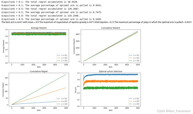
- we test the ε \varepsilon ε-Greedy Algorithm with ε = 0.1 , 0.5 , 0.9 \varepsilon = 0.1,0.5,0.9 ε=0.1,0.5,0.9.
epsilon = np.array([0.1,0.5,0.9])
arms = np.array([Bern_arm(x) for x in arm_mean])
E_greedy,max_i,average_percent,optimal_percent_greedy = plot_algorithm(Greedy,epsilon,arms,arm_mean,num_exper,N,label="$\epsilon$")

print("The maximum of expectation of epsilon-greedy is {:.4f} (epsilon = {})"\
    .format(E_greedy,epsilon[max_i]))
print("The maximum percentage of plays in which the optimal arm is pulled = {:.4f}".format(optimal_percent_greedy))
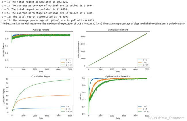
- we test the UCB Algorithem with c = 1 , 5 , 10 c = 1,5,10 c=1,5,10.
c = np.array([1,5,10])
arms = np.array([Bern_arm(x) for x in arm_mean])
E_UCB,max_i,average_percent,optimal_percent_UCB = plot_algorithm(UCB,c,arms,arm_mean,num_exper,N,label="c")

print("The maximum of expectation of UCB is {:.4f} (c = {})"\
    .format(E_UCB,c[max_i]))
print("The maximum percentage of plays in which the optimal arm is pulled = {:.4f}".format(optimal_percent_UCB))
- we test Thompson Sampling.
beta = np.array([[[1,1,1],[1,1,1]],[[601,401,2],[401,601,3]]])
arms = np.array([Bern_arm(x) for x in arm_mean])
E_TS,max_i,average_percent,optimal_percent_TS = plot_algorithm(TS,beta,arms,arm_mean,num_exper,N,label="$beta$")

print("The maximum of expectation of Thompson Sampling is {:.4f} (beta {})"\
    .format(E_TS,max_i+1))
print("The maximum percentage of plays in which the optimal arm is pulled = {:.4f}".format(optimal_percent_TS))
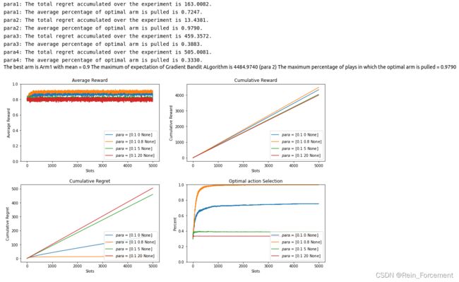
- we test Gradient Bandit Algorithm with baseline b = 0 , 0.8 , 5 , 20 b = 0, 0.8, 5, 20 b=0,0.8,5,20.
# para_list:[step_size, baseline, beta] (default: step_size = 0.1, beta = 1)
step_size = 0.1
para = np.array([[step_size, 0, None], [step_size, 0.8, None], [step_size, 5, None], [step_size, 20, None]])
arms = np.array([Bern_arm(x) for x in arm_mean])
E_Gradient,max_i,average_percent,optimal_percent_gradient = plot_algorithm(Gradient,para,arms,arm_mean,num_exper,N,label="$para$")

print("The maximum of expectation of Gradient Bandit ALgorithm is {:.4f} (para {})"\
    .format(E_Gradient,max_i+1))
print("The maximum percentage of plays in which the optimal arm is pulled = {:.4f}".format(optimal_percent_gradient))
- we test Parameterized Gradient Bandit with constant parameter β = 0.2 , 1 , 2 , 5 \beta = 0.2, 1, 2, 5 β=0.2,1,2,5.
# parameter list:[step_size, baseline, beta] (default: baseline = mean(R_t), step_size = 0.1)
step_size = 0.1
para = np.array([[step_size, None, 0.2], [step_size, None, 1], [step_size, None, 2], [step_size, None, 5]])
arms = np.array([Bern_arm(x) for x in arm_mean])
E_Para_Gradient_const,max_i,average_percent,optimal_percent_para_const = plot_algorithm(Gradient,para,arms,arm_mean,num_exper,N,label="$para$")

print("The maximum of expectation of Parameterized Gradient Bandit Algorithm (beta is a constant) is {:.4f} (para {})"\
    .format(E_Para_Gradient_const,max_i+1))
print("The maximum percentage of plays in which the optimal arm is pulled = {:.4f}".format(optimal_percent_para_const))
-
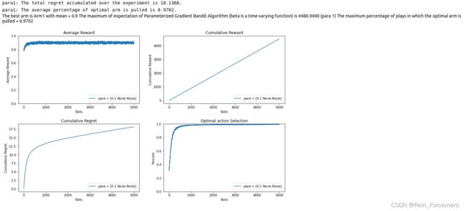
we test Parameterized Gradient Bandit with time-varying parameters β t = l o g ( t ) \beta_t = log(t) βt=log(t).
We choose β t = l o g ( t ) \beta_t = log(t) βt=log(t) as the time-varying parameter because we want to find a monotonically increasing function so that when t t t is small, the model takes more exploration process, and when t t t is large, the model will have more exploitation process.
# parameter list:[step_size, baseline, beta] (default: baseline = mean(R_t), step_size = 0.1)
step_size = 0.1
para = np.array([[step_size, None, None]])
arms = np.array([Bern_arm(x) for x in arm_mean])
E_Para_Gradient_func,max_i,average_percent,optimal_percent_para_func = plot_algorithm(Gradient,para,arms,arm_mean,num_exper,N,label="$para$")

print("The maximum of expectation of Parameterized Gradient Bandit Algorithm (beta is a time-varying function) is {:.4f} (para {})"\
    .format(E_Para_Gradient_func,max_i+1))
print("The maximum percentage of plays in which the optimal arm is pulled = {:.4f}".format(optimal_percent_para_func))
Step 3: Results and Explanations
1. The performance of the three algorithms
Therefore, we compute the oracle value and the expectation rewards of the three respectively:
# Compute the oracle value over N = 5000 turns

arm_mean = [0.9,0.8,0.7]
# number of slots
N = 5000
# number of experiments
num_exper = 1000

oracle_value,max_i = Oracle(arm_mean,N)
print("The oracle value:",oracle_value)
print("Expectation of epsilon-Greedy: {:.4f}".format(E_greedy))
print("Expectation of UCB: {:.4f}".format(E_UCB))
print("Expectation of Thompson: {:.4f}".format(E_TS))
print("Expectation of Gradient Bandit: {:.4f}".format(E_Gradient))
And then we can calculate the gap between the expectation rewards of each algorithm and the oracle value:
print("Gap between epsilon-Greedy and the oracle value: {:.4f}"\
    .format(E_greedy-oracle_value))
print("Gap between UCB and the oracle value: {:.4f}".format(E_UCB-oracle_value))
print("Gap between Thompson and the oracle value: {:.4f}".format(E_TS-oracle_value))
print("Gap between Gradient Bandit and the oracle value: {:.4f}".format(E_Gradient-oracle_value))
print("Percantage of optimal arm of epsion-Greedy: {:.4f}"\
    .format(optimal_percent_greedy))
print("Percantage of optimal arm of UCB: {:.4f}"\
    .format(optimal_percent_UCB))
print("Percantage of optimal arm of TS: {:.4f}"\
    .format(optimal_percent_TS))
print("Percantage of optimal arm of Gradient: {:.4f}"\
    .format(optimal_percent_gradient))
From the result above, we can find that the Thompson Sampling has the least gap between the oracle value, the largest cumulative reward and the largest percentage of optimal arm. So, Thompson Sampling is the best among the three algorithm.
And we can also use the graphs to compare the performance of the three algorithm:
def compare(algorithm, para, arms, num_exper, num_slot):

    fig,axes = plt.subplots(1,2,figsize=[15,6])
    cumulative_reward = dict()

    for i in range(len(algorithm)):
        if algorithm[i] == Greedy or algorithm[i] == UCB:
            #run the algorithm
            algo = algorithm[i](para[i])
            if(algorithm[i] == Greedy):
                algo_name = "Greedy"
            else:
                algo_name = "UCB"
            chosen_arm,average_reward,cum_reward = \
                run_algorithm(algo,arms,num_exper,num_slot)

            #plot the average reward
            axes[0].plot(average_reward,label=algo_name)
            axes[0].set_xlabel("Slots")
            axes[0].set_ylabel("Average Reward")
            axes[0].set_title("Average Reward")
            axes[0].legend(loc="lower right")
            axes[0].set_ylim([0, 1.0])

            #plot the cumulative reward
            axes[1].plot(cum_reward,label=algo_name)
            axes[1].set_xlabel("Slots")
            axes[1].set_ylabel("Cumulative Reward")
            axes[1].set_title("Cumulative Reward")
            axes[1].legend(loc="lower right")

            cumulative_reward[algo_name] = cum_reward[num_slot-1]

        elif algorithm[i] == TS:
            #run the algorithm
            algo = algorithm[i](para[i][0],para[i][1])
            algo_name = "TS"
            chosen_arm,average_reward,cum_reward = \
                run_algorithm(algo,arms,num_exper,num_slot)

            #plot the average reward
            axes[0].plot(average_reward,label=algo_name)
            axes[0].set_xlabel("Slots")
            axes[0].set_ylabel("Average Reward")
            axes[0].set_title("Average Reward")
            axes[0].legend(loc="lower right")
            axes[0].set_ylim([0.0, 1.0])

            #plot the cumulative reward
            axes[1].plot(cum_reward,label=algo_name)
            axes[1].set_xlabel("Slots")
            axes[1].set_ylabel("Cumulative Reward")
            axes[1].set_title("Cumulative Reward")
            axes[1].legend(loc="lower right")

            cumulative_reward[algo_name] = cum_reward[num_slot-1]

        elif algorithm[i] == Gradient:
            #run the algorithm
            algo = algorithm[i](para[i][0], para[i][1], para[i][2])
            algo_name = "Gradient"
            chosen_arm,average_reward,cum_reward = \
                run_algorithm(algo,arms,num_exper,num_slot)

            #plot the average reward
            axes[0].plot(average_reward,label=algo_name)
            axes[0].set_xlabel("Slots")
            axes[0].set_ylabel("Average Reward")
            axes[0].set_title("Average Reward")
            axes[0].legend(loc="lower right")
            axes[0].set_ylim([0, 1.0])

            #plot the cumulative reward
            axes[1].plot(cum_reward,label=algo_name)
            axes[1].set_xlabel("Slots")
            axes[1].set_ylabel("Cumulative Reward")
            axes[1].set_title("Cumulative Reward")
            axes[1].legend(loc="lower right")

            cumulative_reward[algo_name] = cum_reward[num_slot-1]

    plt.show()
    optimal_algo = max(cumulative_reward, key=cumulative_reward.get)
    print("The optimal algorithm with the most cumulative reward is {}".format(optimal_algo))
    print("The maximum of cumulative reward is {:.4f}".format(cumulative_reward[optimal_algo]))
algo = [Greedy, UCB, TS, Gradient]
para = np.array([0.1,1,[[1,1,1],[1,1,1]],[0.1, None, 2]])
arms = np.array([Bern_arm(x) for x in arm_mean])

compare(algo,para,arms,num_exper,N)
According to the result of the graph, we can also find that the Thompson Sampling(with para: { ( α 1 , β 1 ) = ( 1 , 1 ) , ( α 2 , β 2 ) = ( 1 , 1 ) , ( α 3 , β 3 ) = ( 1 , 1 ) (\alpha_1,\beta_1)=(1,1),(\alpha_2,\beta_2)=(1,1),(\alpha_3,\beta_3)=(1,1) (α1,β1)=(1,1),(α2,β2)=(1,1),(α3,β3)=(1,1)}) has the best performance among the three algorithms.
2. The impact of the parameter
1 ∘ 1^{\circ} 1∘ ε \varepsilon ε
The simulation above shows that when ε = 0.2 \varepsilon = 0.2 ε=0.2, the ε \varepsilon ε-Greedy algorithm performes best, so we can suppose that ε \varepsilon ε has negative correlation with the expected correlation.
Then we prove the suppose by the definition of ε \varepsilon ε-Greedy in an intuitive degree:
The value of ε \varepsilon ε decides the probability of exploration, the larger ε \varepsilon ε is, the more exploration occurs. In this question, exploiting will bring out more rewards than exploration, so ε \varepsilon ε has negative correlation with the expected correlation is obvious intuitively.
2 ∘ 2^{\circ} 2∘ c
The simulation above shows that when c = 1 c = 1 c=1, the UCB algorithm performes best, so we can suppose that c has negative correlation with the expected correlation.
Then we prove the suppose by the definition of UCB in an intuitive degree:
Since Q ^ ( a ) + c − l o g t 2 N t ( a ) \hat{Q}(a)+c\sqrt{\frac{-logt}{2N_t(a)}} Q^(a)+c2Nt(a)−logt is the upper bound of value function Q ( a ) Q(a) Q(a), c indicates how much we trust the existing estimated value function of an action Q ^ ( a ) \hat{Q}(a) Q^(a). The larger the value of c, the more uncertain we are about the existing estimated value function, which means we need to more exploration to validate the estimated value function.
The value of c c c represents the weight of exploration, the larger c c c is, the more weight exploration has. In this question, exploiting will bring out more rewards than exploration, so c has negative correlation with the expected correlation is obvious intuitively.
3 ∘ 3^\circ 3∘ α j , β j \alpha_j, \beta_j αj,βj
The simulation above shows that when b e t a 1 : ( α 1 , β 1 ) = ( α 2 , β 2 ) = ( α 3 , β 3 ) = ( 1 , 1 ) beta1: (\alpha_1,\beta_1) = (\alpha_2,\beta_2) = (\alpha_3,\beta_3) = (1,1) beta1:(α1,β1)=(α2,β2)=(α3,β3)=(1,1), the Thompson Sampling algorithm performes best.
Then we give an explanation by the definition of Beta Distribution in an intuitive degree:
For Beta distribution, α \alpha α means the prior number of success, β \beta β means the prior number of failure, the rate of success: α α + β \frac{\alpha}{\alpha+\beta} α+βα is its mean. When the expectation of one arm is larger, the probability to choose the arm is larger. But if α + β \alpha+\beta α+β is large, the variance of Beta Distribution is small.
Thus, α j , β j \alpha_j, \beta_j αj,βj is in fact a prior success and failure times, and have properties as below:
(1) the larger the mean α α + β \frac{\alpha}{\alpha+\beta} α+βα, the closer the center of the probability density distribution is to 1, and the random numbers generated according to this probability distribution are said to be close to 1, and vice versa. In this case, arms with high means are more likely to be chosen
(2) The larger the value α + β \alpha+\beta α+β, the narrower the distribution, that is, the higher the concentration and lower the variance, and the random numbers generated in this way are closer to the center position, which can also be seen from the variance formula. In this case, arms with high variance is more likely to be explored and updated.
4 ∘ 4^\circ 4∘ baseline b b b
The main purpose of introducing the baseline is to reduce the variance of algorithm and make the algorithm easier to converge. Because the introduction of the baseline makes the gap between the reward in different states smaller, that is, the global variance becomes smaller.
We often regard R ^ ( t ) \hat{R}(t) R^(t) as the baseline, which means that R t ( a ) R_t(a) Rt(a) being greater than R ^ ( t ) \hat{R}(t) R^(t) corresponds to a lifting effectV(s) on π t ( a ) \pi_t(a) πt(a) , R t ( a ) R_t(a) Rt(a) being less than R ^ ( t ) \hat{R}(t) R^(t) corresponds to a reducing effect on π t ( a ) \pi_t(a) πt(a).
5 ∘ 5^\circ 5∘ β \beta β (Gradient)
The introduction of β \beta β into the softmax function can make the gap of probability of different action π t ( a ) \pi_t(a) πt(a) corresponding to the numerically limited preference function H t ( a ) H_t(a) Ht(a) larger, especially when the β \beta β is large.
The introduction of the parameter β \beta β will make the action with a larger preference function to be selected more preferentially. A large value of β \beta β will reduce the probability of exploration, and is more inclined to exploition. If β → 0 \beta \to 0 β→0, it will only explore. If β → ∞ \beta \to \infty β→∞, it will only exploit.
III Understanding of the Exploration-Exploiting Trade-Off
Assume a case that when you plan to eat at a certain resturant, you can choose to eat the favourite dish you have known, and you can also try some new dishes which you have not eaten before. The former is the exploiting, and the latter is the exploration.
In the bandit algorithms, the exploiting strategy means to draw the arm that seem best based on past outcomes, and the exploration strategy is to pick choices not yet tried out (or not tried enough).
We need to explore because the given information is valuable. But we can do no exploration at all,focusing on the short-term returns. We need to occasionally explore at random: some short-term sacrifice may bring out more long-term reward, because you cannot make sure that the one we exploit is the global optimum, rather than the local optimum. So, we need to use the exploration strategy in this problem to find other possibilities. Otherwise, we may get stuck in a local optimum, and will be unable to find the global optimum.
IV. Dependent Case
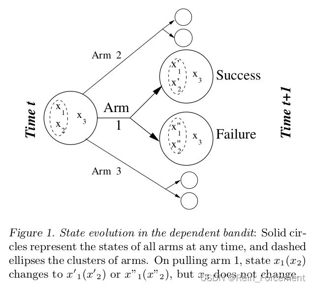
Formally, the dependent bandit problem is defined as follows. There is a slot machine with N N N arms that are grouped into K K K known clusters. Each arm i i i has a fixed but unknown success probability θ i θ_i θi . Let [ i ] [i] [i] denote the cluster of arm i i i. Let C [ i ] C_{[i]} C[i] be the set of all arms in cluster [ i ] [i] [i] (including i i i itself), and let C [ i ] − i = C [ i ] − i C_{[i]}^{-i} = C_{[i] - {i}} C[i]−i=C[i]−i.
Firstly, we assume that the dependencies among arms in a cluster can be described by a generative model. The form of the generative model is known but its parameters are unknown. In particular, let s i ( t ) s_i(t) si(t) be the number of times arm i i i generated a unit reward when pulled (“successes”), and f i ( t ) f_i(t) fi(t) the number of “failures.” Then, for each arm i i i in cluster [ i ] [i] [i], we assume that
s i ( t ) ∣ θ i ∼ B e r n ( θ i ) s_i(t) | \theta_i \sim Bern(\theta_i) si(t)∣θi∼Bern(θi)
θ i ∼ η ( π [ i ] ) \theta_i \sim \eta(\pi_{[i]}) θi∼η(π[i])
where η ( . ) \eta(.) η(.) is a probability distribution and π [ i ] \pi_{[i]} π[i] is the parameter set for cluster [ i ] [i] [i]. Intuitively, π C \pi_C πC abstracts out the dependence of arms in cluster C C C on each other; given π C \pi_C πC , each arm is independent of all other arms in other clusters.
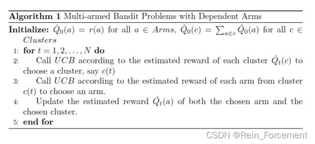
Then we can discuss the problem on a per-cluster basis, because arms in different clusters is independent. The pseudocode is as below:
By first dividing the arm into different clusters and using the UCB algorithm twice, first find the current optimal cluster, and then find the optimal arm from this cluster. Finally, the reward is updated through the UCB algorithm. We can estimate the optimal action of dependent arm bandit problems.
V. Why sublinear regret is the performance threshold
The cause of sublinear regret being the performance threshold is mainly due to its the influence on the optimal strategy.
According to regret decomposition rule, cumulative regret L t = ∑ a ∈ A E ( N t ( a ) ) Δ a L_t = \sum_{a\in A}E(N_t(a))\Delta_a Lt=∑a∈AE(Nt(a))Δa. If an algorithm has an linear regret, that is L t = Θ ( n ) L_t = \Theta(n) Lt=Θ(n), we have ∑ a ∈ A E ( N t ( a ) ) Δ a = Θ ( t ) \sum_{a\in A}E(N_t(a))\Delta_a = \Theta(t) ∑a∈AE(Nt(a))Δa=Θ(t). And because ∑ a ∈ A E ( N t ( a ) ) = E ( ∑ a ∈ A N t ( a ) ) = 1 \sum_{a\in A}E(N_t(a)) = E(\sum_{a\in A}N_t(a)) = 1 ∑a∈AE(Nt(a))=E(∑a∈ANt(a))=1, we can then deduce that the mean value of the gap between the reward obtained by each pull and the optimal reward will be a number greater than 0 and the mean of opportunity loss: E ( V ∗ − Q t ( a ) ) = Θ ( 1 ) E(V^* - Q_t(a)) = \Theta(1) E(V∗−Qt(a))=Θ(1) for each pull t t t. In other word, when t → ∞ t \to \infty t→∞, the probability of choose the optimal will not be converge to 1, which means the learner cannot get the optimal choice accurately enough.
For example, The total regret of ε − g r e e d y \varepsilon-greedy ε−greedy: L t ≥ ε t ∣ A ∣ ∑ a ∈ A Δ a L_t \geq \frac{\varepsilon t}{|A|}\sum_{a\in A}\Delta_a Lt≥∣A∣εt∑a∈AΔa, and the average regret R t ‾ ≥ ε ∣ A ∣ ∑ a ∈ A Δ a = Θ ( 1 ) \overline{R_t} \geq \frac{\varepsilon}{|A|}\sum_{a\in A}\Delta_a = \Theta(1) Rt≥∣A∣ε∑a∈AΔa=Θ(1) and the result will not converge to 0. As a consequence, when t → ∞ t \to \infty t→∞, although we already have high confidence in the optimal choice, we still have the probability of ε × ∣ A ∣ − 1 ∣ A ∣ \varepsilon\times \frac{|A|-1}{|A|} ε×∣A∣∣A∣−1 not choose the optimal and the probability will not converge to 0 0 0.
When it comes to algorithms with sublinear regret such as U C B UCB UCB: ( L t ≤ 8 l o g t ∑ a ∈ A Δ a L_t \leq 8logt\sum_{a\in A}\Delta_a Lt≤8logt∑a∈AΔa), we can find policy π \pi π such that regret R t → 0 R_t \to 0 Rt→0 when time t → ∞ t \to \infty t→∞. In this case, the learner will choose the optimal action almost all of the time as the horizon t t t tends to infinity.
In conclusion, after considering the choice of the optimal action, sublinear regret is the performance threshold is mainly due to its the influence on the optimal strategy.
Reference
[1] epsilon-Greedy Algorithm
[2] The Multi-Armed Bandit Problem and Its Solutions
[3] Bayesian A/B testing with Thompson sampling
[4] 关于Multi-Armed Bandit(MAB)问题及算法
[5] Sandeep Pandey Deepayan Chakrabarti Deepak Agarwal “Multi-armed Bandit Problems with Dependent Arms”
[6] Tor Lattimore and Csaba Szepesvári “Bandit Algorithms”

