How to Lift Performance With Learning Rate Schedules

Training a neural network or large deep learning model is a difficult optimization task.The classical algorithm to train neural networks is called stochastic gradient descent. It has been well established that you can achieve increased performance and faster training on some problems by using a learning rate that changes during training. In this lesson you will discover how you can use di↵erent learning rate schedules for your neural network models in Python using the Keras deep learning library. After completing this lesson you will know:

• The benefit of learning rate schedules on lifting model performance during training.
• How to configure and evaluate a time-based learning rate schedule.
• How to configure and evaluate a drop-based learning rate schedule.

1.1 Learning Rate Schedule For Training Models

 Adapting the learning rate for your stochastic gradient descent optimization procedure can increase performance and reduce training time. Sometimes this is called learning rate annealing or adaptive learning rates.Here we will call this approach a learning rate schedule, were the default schedule is to use a constant learning rate to update network weights for each training epoch.

        The simplest and perhaps most used adaptation of learning rates during training are techniques that reduce the learning rate over time. These have the benefit of making large changes at the beginning of the training procedure when larger learning rate values are used, and decreasing the learning rate such that a smaller rate and therefore smaller training updates are made to weights later in the training procedure. This has the effect of quickly learning good weights early and fine tuning them later. Two popular and easy to use learning rate schedules are as follows:

• Decrease the learning rate gradually based on the epoch.
• Decrease the learning rate using punctuated large drops at specific epochs.

Next, we will look at how you can use each of these learning rate schedules in turn with Keras.

1.2  Ionosphere Classification Dataset

The Ionosphere binary classification problem is used as a demonstration in this lesson. The dataset describes radar returns where the target was free electrons in the ionosphere. It is a binary classification problem where positive cases (g for good) show evidence of some type of structure in the ionosphere and negative cases (b for bad) do not. It is a good dataset for practicing with neural networks because all of the inputs are small numerical values of the same scale. There are 34 attributes and 351 observations.

        State-of-the-art results on this dataset achieve an accuracy of approximately 94% to 98% accuracy using 10-fold cross validation1. The dataset is available within the code bundle provided with this book. Alternatively, you can download it directly from the UCI Machine Learning repository2. Place the data file in your working directory with the filename ionosphere.csv. You can learn more about the ionosphere dataset on the UCI Machine Learning Repository website3.

• http://www.is.umk.pl/projects/datasets.html#Ionosphere
• http://archive.ics.uci.edu/ml/machine-learning-databases/ionosphere/ionosphere.data
• https://archive.ics.uci.edu/ml/datasets/Ionosphere

1.3  Time-Based Learning Rate Schedule

Keras has a time-based learning rate schedule built in. The stochastic gradient descent optimization algorithm implementation in the SGD class has an argument called decay. This argument is used in the time-based learning rate decay schedule equation as follows:

When the decay argument is zero (the default), this has no e↵ect on the learning rate (e.g. 0.1).

# Example Calculating Learning Rate Without Decay.

LearningRate = 0.1 * 1/(1 + 0.0 * 1)

LearningRate = 0.1

When the decay argument is specified, it will decrease the learning rate from the previous epoch by the given fixed amount. For example, if we use the initial learning rate value of 0.1 and the decay of 0.001, the first 5 epochs will adapt the learning rate as follows:

# Output of Calculating Learning Rate With Decay.

Epoch Learning Rate

1         0.1

2         0.0999000999

3         0.0997006985

4         0.09940249103

5         0.09900646517

 Extending this out to 100 epochs will produce the following graph of learning rate (y-axis) versus epoch (x-axis):

 

# Example of A Good Default Decay Rate.

Decay = LearningRate / Epochs

Decay = 0.1 / 100

Decay = 0.001

         The example below demonstrates using the time-based learning rate adaptation schedule in Keras. A small neural network model is constructed with a single hidden layer with 34 neurons and using the rectifier activation function. The output layer has a single neuron and uses the sigmoid activation function in order to output probability-like values. The learning rate for stochastic gradient descent has been set to a higher value of 0.1. The model is trained for 50 epochs and the decay argument has been set to 0.002, calculated as 0.1 50 . Additionally, it can be a good idea to use momentum when using an adaptive learning rate. In this case we use a momentum value of 0.8. The complete example is listed below.

# Time Based Learning Rate Decay
import pandas as pd
import numpy as np
from keras.models import Sequential
from keras.layers import Dense
from tensorflow.keras.optimizers import SGD
from sklearn.preprocessing import LabelEncoder

# fix random seed for reproducibility
seed = 7
np.random.seed(seed)
# load dataset
dataframe = pd.read_csv("ionosphere.csv", header=None)
dataset = dataframe.values

# split into input (X) and output(Y) variables
X = dataset[:,0:34].astype(float)
Y = dataset[:,34]

# encode class values as integers
encoder = LabelEncoder()
encoder.fit(Y)
Y = encoder.transform(Y)

# create model
model = Sequential()
model.add(Dense(34, input_dim=34, kernel_initializer='normal',activation='relu'))
model.add(Dense(1,kernel_initializer='normal',activation='sigmoid'))
# Compile model
epochs = 50
learning_rate = 0.1
decay_rate = learning_rate / epochs
momentum = 0.8
sgd = SGD(lr=learning_rate, momentum=momentum, decay=decay_rate, nesterov=False)
model.compile(loss='binary_crossentropy', optimizer=sgd, metrics=['accuracy'])
# Fit the model
model.fit(X, Y, validation_split=0.33, epochs=epochs, batch_size=28, verbose=2)

         The model is trained on 67% of the dataset and evaluated using a 33% validation dataset. Running the example shows a classification accuracy of 99.14%. This is higher than the baseline of 95.69% without the learning rate decay or momentum.

1.4 Drop-Based Learning Rate Schedule

Another popular learning rate schedule used with deep learning models is to systematically drop the learning rate at specific times during training. Often this method is implemented by dropping the learning rate by half every fixed number of epochs. For example, we may have an initial learning rate of 0.1 and drop it by a factor of 0.5 every 10 epochs. The first 10 epochs of training would use a value of 0.1, in the next 10 epochs a learning rate of 0.05 would be used, and so on. If we plot out the learning rates for this example out to 100 epochs you get the graph below showing learning rate (y-axis) versus epoch (x-axis).

 We can implement this in Keras using the LearningRateScheduler callback4 when fitting the model. The LearningRateScheduler callback allows us to define a function to call that takes the epoch number as an argument and returns the learning rate to use in stochastic gradient descent. When used, the learning rate specified by stochastic gradient descent is ignored. In the code below, we use the same example before of a single hidden layer network on the Ionosphere dataset. A new step decay() function is defined that implements the equation:

 

        Where InitialLearningRate is the learning rate at the beginning of the run, EpochDrop is how often the learning rate is dropped in epochs and DropRate is how much to drop the learning rate each time it is dropped.

# Example of Drop-Based Learning Rate Decay
# Drop-Based Learning Rate Decay
import pandas as pd
import numpy as np
import math
from keras.models import Sequential
from keras.layers import Dense
from tensorflow.keras.optimizers import SGD
from sklearn.preprocessing import LabelEncoder
from keras.callbacks import LearningRateScheduler

# learning rate schedule
def step_decay(epoch):
    initial_lrate = 0.1
    drop = 0.5
    epochs_drop = 10.0
    lrate = initial_lrate * math.pow(drop, math.floor((1+epoch)/epochs_drop))
    return lrate
# fix random seed for reproducibility
seed = 7
np.random.seed(seed)

# load dataset
dataframe = pd.read_csv("ionosphere.csv",header=None)
dataset = dataframe.values

# split into input(X) and output (Y) variables
X = dataset[:,0:34].astype(float)
Y = dataset[:,34]

# encode class values as integers
encoder = LabelEncoder()
encoder.fit(Y)
Y = encoder.transform(Y)

# create model
model = Sequential()
model.add(Dense(34, input_dim=34,kernel_initializer='normal',activation='relu'))
model.add(Dense(1, kernel_initializer='normal',activation='sigmoid'))

# compile model
sgd = SGD(lr=0.0, momentum=0.9, decay=0.0, nesterov=False)
model.compile(loss='binary_crossentropy',optimizer=sgd,metrics=['accuracy'])

# learning schedule callback
lrate = LearningRateScheduler(step_decay)
callbacks_list = [lrate]
# Fit the model
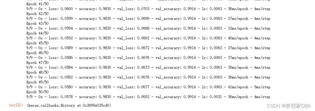
model.fit(X, Y, validation_split=0.33, epochs=50, batch_size=28,callbacks=callbacks_list, verbose=2)

         Running the example results in a classification accuracy of 99.14% on the validation dataset, again an improvement over the baseline for the model on this dataset.

1.5 Tips for Using Learning Rate Schedules

This section lists some tips and tricks to consider when using learning rate schedules with neural networks.

• Increase the initial learning rate. Because the learning rate will decrease, start with a larger value to decrease from. A larger learning rate will result in a lot larger changes to the weights, at least in the beginning, allowing you to benefit from fine tuning later.
• Use a large momentum. Using a larger momentum value will help the optimization algorithm to continue to make updates in the right direction when your learning rate shrinks to small values.
• Experiment with different schedules. It will not be clear which learning rate schedule to use so try a few with different configuration options and see what works best on your problem. Also try schedules that change exponentially and even schedules that respond to the accuracy of your model on the training or test datasets.

1.6 Summary

In this lesson you discovered learning rate schedules for training neural network models. You learned:

• The benefits of using learning rate schedules during training to lift model performance.
• How to configure and use a time-based learning rate schedule in Keras.
• How to develop your own drop-based learning rate schedule in Keras