计算机视觉可解释性——CAM热力图的研读与复现

论文题目：Learning Deep Features for Discriminative Localization
(Class Activation Mapping)
论文地址：https://arxiv.org/pdf/1512.04150.pdf
完整代码：https://github.com/metalbubble/CAM
—————————————————————————————————

论文研读

问题：
1.以前的全监督的CNN方法，会进行标签标注，导致浪费大量的人力与时间成本。

2.全连接层
a) 全连接层被用作分类，所以导致在此层的定位能力丢失（卷积神经网络的全连接层会将最后一层的特征图拉平来和全连接层相连，这样破坏了空间位置信息就破坏了，而全局平均池化层不需要破话空间结构）。
b) 全连接层有大量参数，计算成本高。

主要贡献：
1.使用弱监督目标定位
2.CNN内部表示的可视化

流程图:
方法：

使用全局平均池化GAP（Global Average Pooling）与GMP（Global Max Pooling）的区别：
GMP能够帮助卷积神经网络找到一个不同的区域，而GAP则能够精确的找到目标在图像中的范围。对于GAP来说，所有较高的值都会对整体训练有比较大的贡献（取平均值）。对于GMP来说，只有最大值的那个点会产生贡献。作者在ImageNet 上测试了两种全局池化方式，发现分类结果相近，但是定位的结果GAP远远超过GMP。

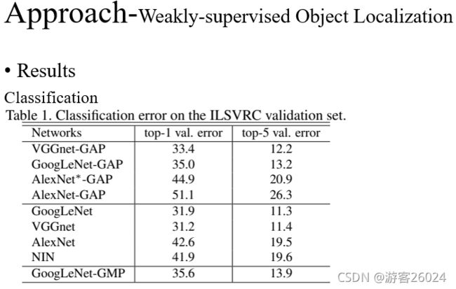
从表1可得，我们的分类error相对于使用全连接层的error来说，相差1-2个百分点。比如VGGnet 31.2 top1 error vs VGGnet-GAP 33.4 top1 error| AlexNet 42.6 top1 error vs AlexNet*-GAP 44.9 top1 error (加*代表在替换fc层之后，又增加2层卷积层，再加了GAP层)。我们GAP的分类结果相比与GMP分类来说，效果更好（理由如上）。

从表2可得，我们使用全局平均池化的方法定位 比 反向传播的CNN方法定位、全局最大池化的方法定位 效果更好，其中GoogLeNet-GAP最佳为56.40 top1 error | 43.00 top5 error

从表3可得，我们使用的弱监督定位方法 比 全监督定位方法 想过更好，其中GoogLeNet-GAP(启发式 [修改了 bbox] ) 为 37.1 top5 error

上图表示，每个BackBone 生成的不同定位方法，使用热力图展示，其中BackBone的VGG-GAP效果最好。

从图6可得，其中在原图上现实的绿框为Ground Truth,红框为预测的结果。a)为使用BackBone（GooLeNet-GAP）的结果，b)为GoogLeNet-GAP（upper two）与 the backpropagation using AlexNet (lower two)的结果。

从表5可得，使用不同的数据集与BackBone产生的精度结果。

从图8可得，使用不同数据集与GoogLeNet-GAP产生的定位结果。

从表4可得，在CUB200数据集与GoogLeNet-GAP产生的细粒度分类性能，并能成功定位重要图像区域。

从图7可得，使用弱监督定位方法产生的bbox。

从图9可得，不同场景下的带信息的目标效果。

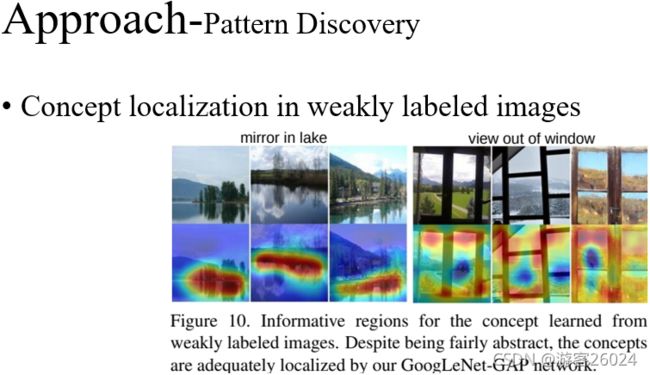
从图10可得，在弱标签图像的概念定位(镜子、湖等)。

从图11可得，弱监督文本检测的结果。

从图12可得，图像问答的定位结果。

从图13可得，特殊类别单元的可视化，Mask结果。

—————————————————————————————————

代码复现

import os
import cv2
from PIL import Image
from torchvision import models, transforms
from torch.autograd import Variable
from torch.nn import functional as F
import numpy as np
from torchvision.models.densenet import densenet161
import json

# input image 
# 使用本地的图片与本地的标签
labels_file = 'imagenet-simple-labels.json'
image_path = "31.jpg"

# networks such as Googlenet, ResNet,Densent already use global average pooling at the end,
# so CAM could be used directly.

# 选择使用的网络
model_id = 2

# 选择网络
if model_id == 1:
    net = models.squeezenet1_1(pretrained=True)
    finalconv_name = 'features'

elif model_id == 2:
    net = models.resnet18(pretrained=True)
    finalconv_name = 'layer4'
elif model_id == 3:
    net = densenet161()
    finalconv_name = "features"

# 有固定参数作用，如norm的参数
net.eval()

# 获取特定层的feature map
# hook the feature extractor
features_blobs = []


def hook_feature(module, input, output):
    features_blobs.append(output.data.cpu().numpy())


net._modules.get(finalconv_name).register_forward_hook(hook_feature)

# get the softmax weight
# 倒数第二层
params = list(net.parameters()) # 将参数变换为列表
weight_softmax = np.squeeze(params[-2].data.numpy()) # 提取softmax层的参数

# 生成CAM图的函数，完成权重和feature相乘操作
def returnCAM(feature_conv, weight_softmax, class_idx):
    # generate the class activation maps upsample to 256x256
    size_upsample = (256, 256)
    bc, nc, h, w = feature_conv.shape
    output_cam = []
    # class_idx为预测分数较大的类别数字表示的数组，一张图片中有N个类物体，则数组中N个元素
    for idx in class_idx:
        # 回到GAP的值
        # weight_softmax中预测为第idx类的参数w乘以feature_map,为了相乘reshape map的形状
        cam = weight_softmax[idx].dot(feature_conv.reshape(nc, h * w))
        #将feature_map的形状reshape回去
        cam = cam.reshape(h, w)
				
				# 归一化操作（最小值为0，最大值为1）
        # np.min 返回数组的最小值或沿轴的最小值
        cam = cam - np.min(cam)
        cam_img = cam / np.max(cam)
			
				# 转换为图片255的数据
        # np.uint8() Create a data type object.
        cam_img = np.uint8(255 * cam_img)

			 # resize 图片尺寸与输入图片一致
        output_cam.append(cv2.resize(cam_img, size_upsample))

    return output_cam

# 数据处理，先缩放尺寸到(224,224)，再变换数据类型为tensor,最后normalize
normalize = transforms.Normalize(
    mean=[0.485, 0.456, 0.406],
    std=[0.229, 0.224, 0.225]
)

preprocess = transforms.Compose([
    transforms.Resize((224, 224)),
    transforms.ToTensor(),
    normalize
])
image_path = os.path.expanduser(image_path)
img_pil = Image.open(image_path)
img_pil.save('test.jpg')
# 将图片数据处理成所需要的可用数据 tensor
img_tensor = preprocess(img_pil)
# 处理图片为Variable数据
img_variable = Variable(img_tensor.unsqueeze(0))
#将图片输入网络得到预测类别分数
logit = net(img_variable)
# 分类标签列表，并存储在classes(数字类别，类别名称)
with open(labels_file) as f:
    classes = json.load(f)
    
# 使用softmax打分
h_x = F.softmax(logit, dim=1).data.squeeze()
# 对分类的预测类别分数排序，输出预测值和在列表中的位置
probs, idx = h_x.sort(0, True)

# 转换数据类型
probs = probs.numpy()
idx = idx.numpy()

# 输出预测分数排名在前5个类别的预测分数和对应的类别名称
for i in range(0, 5):
    print('{:.3f} -> {}'.format(probs[i], classes[idx[i]]))

# 输出与图片尺寸一致的CAM图片
# generate class activation mapping for the top1 prediction
CAMs = returnCAM(features_blobs[0], weight_softmax, [idx[0]])

# render the CAM and output
print("output CAM.jpg")

# 将图片和CAM拼接在一起展示定位结果
img = cv2.imread("31.jpg")
height, width, _ = img.shape
# 生成热力图
heatmap = cv2.applyColorMap(cv2.resize(CAMs[0], (width, height)), cv2.COLORMAP_JET)
result = cv2.addWeighted(img, 0.3, heatmap, 0.5, 0)
cv2.imwrite('CAM.jpg', result)
cv2.imshow("heatmap", result)
cv2.waitKey(0)
cv2.destroyAllWindows()

注意：
1.本地标签的下载 点击我

2.使用残差网络作为BackBone，效果更好

效果展示
原图：
___________________________________________________________
CAM热力图展示：
___________________________________________________________

控制台现实最大的前五个类别的置信度：