数据挖掘实战:二手车交易价格预测之特征工程
特征工程用于对特征进行进一步分析,并对数据进行处理
常见特征工程包括:
- 异常处理:
通过箱线图(或 3-Sigma)分析删除异常值;
BOX-COX 转换(处理有偏分布);
长尾截断; - 特征归一化/标准化:
标准化(转换为标准正态分布);
归一化(抓换到 [0,1] 区间);
针对幂律分布,可以采用公式: - 数据分桶:
等频分桶;
等距分桶;
Best-KS 分桶(类似利用基尼指数进行二分类);
卡方分桶; - 缺失值处理:
不处理(针对类似 XGBoost 等树模型);
删除(缺失数据太多);
插值补全,包括均值/中位数/众数/建模预测/多重插补/压缩感知补全/矩阵补全等;
分箱,缺失值一个箱; - 特征构造:
构造统计量特征,报告计数、求和、比例、标准差等;
时间特征,包括相对时间和绝对时间,节假日,双休日等;
地理信息,包括分箱,分布编码等方法;
非线性变换,包括 log/ 平方/ 根号等;
特征组合,特征交叉;
( 1+1+ ) - 特征筛选
过滤式(filter):先对数据进行特征选择,然后在训练学习器,常见的方法有 Relief/方差选择发/相关系
数法/卡方检验法/互信息法;
包裹式(wrapper):直接把最终将要使用的学习器的性能作为特征子集的评价准则,常见方法有
LVM(Las Vegas Wrapper) ;
嵌入式(embedding):结合过滤式和包裹式,学习器训练过程中自动进行了特征选择,常见的有
lasso 回归; - 降维
PCA/ LDA/ ICA;
特征选择也是一种降维
导入数据
import pandas as pd
import numpy as np
import matplotlib
import matplotlib.pyplot as plt
import seaborn as sns
from operator import itemgetter
%matplotlib inline
train = pd.read_csv('used_car_train_20200313.csv', sep=' ')
test = pd.read_csv('used_car_testA_20200313.csv', sep=' ')
print(train.shape)
print(test.shape)
(150000, 31)
(50000, 30)
train.head()
| SaleID | name | regDate | model | brand | bodyType | fuelType | gearbox | power | kilometer | ... | v_5 | v_6 | v_7 | v_8 | v_9 | v_10 | v_11 | v_12 | v_13 | v_14 | |
|---|---|---|---|---|---|---|---|---|---|---|---|---|---|---|---|---|---|---|---|---|---|
| 0 | 0 | 736 | 20040402 | 30.0 | 6 | 1.0 | 0.0 | 0.0 | 60 | 12.5 | ... | 0.235676 | 0.101988 | 0.129549 | 0.022816 | 0.097462 | -2.881803 | 2.804097 | -2.420821 | 0.795292 | 0.914762 |
| 1 | 1 | 2262 | 20030301 | 40.0 | 1 | 2.0 | 0.0 | 0.0 | 0 | 15.0 | ... | 0.264777 | 0.121004 | 0.135731 | 0.026597 | 0.020582 | -4.900482 | 2.096338 | -1.030483 | -1.722674 | 0.245522 |
| 2 | 2 | 14874 | 20040403 | 115.0 | 15 | 1.0 | 0.0 | 0.0 | 163 | 12.5 | ... | 0.251410 | 0.114912 | 0.165147 | 0.062173 | 0.027075 | -4.846749 | 1.803559 | 1.565330 | -0.832687 | -0.229963 |
| 3 | 3 | 71865 | 19960908 | 109.0 | 10 | 0.0 | 0.0 | 1.0 | 193 | 15.0 | ... | 0.274293 | 0.110300 | 0.121964 | 0.033395 | 0.000000 | -4.509599 | 1.285940 | -0.501868 | -2.438353 | -0.478699 |
| 4 | 4 | 111080 | 20120103 | 110.0 | 5 | 1.0 | 0.0 | 0.0 | 68 | 5.0 | ... | 0.228036 | 0.073205 | 0.091880 | 0.078819 | 0.121534 | -1.896240 | 0.910783 | 0.931110 | 2.834518 | 1.923482 |
5 rows × 31 columns
train.columns
Index(['SaleID', 'name', 'regDate', 'model', 'brand', 'bodyType', 'fuelType',
       'gearbox', 'power', 'kilometer', 'notRepairedDamage', 'regionCode',
       'seller', 'offerType', 'creatDate', 'price', 'v_0', 'v_1', 'v_2', 'v_3',
       'v_4', 'v_5', 'v_6', 'v_7', 'v_8', 'v_9', 'v_10', 'v_11', 'v_12',
       'v_13', 'v_14'],
      dtype='object')
test.columns
Index(['SaleID', 'name', 'regDate', 'model', 'brand', 'bodyType', 'fuelType',
       'gearbox', 'power', 'kilometer', 'notRepairedDamage', 'regionCode',
       'seller', 'offerType', 'creatDate', 'v_0', 'v_1', 'v_2', 'v_3', 'v_4',
       'v_5', 'v_6', 'v_7', 'v_8', 'v_9', 'v_10', 'v_11', 'v_12', 'v_13',
       'v_14'],
      dtype='object')
删除异常值
# 这里封装一个异常值处理的代码,可供后续调用。
def outliers_proc(data, col_name, scale=3):
    """
    用于清洗异常值,默认用 box_plot(scale=3)进行清洗
    :param data: 接收 pandas 数据格式
    :param col_name: pandas 列名
    :param scale: 尺度
    :return:
    """

    def box_plot_outliers(data_ser, box_scale):
        """
        利用箱线图去除异常值
        :param data_ser: 接收 pandas.Series 数据格式
        :param box_scale: 箱线图尺度,
        :return:
        """
        # quantile 是分位函数,相当于取每列属性取值范围的3/4位置的值减去1/4位置的值,乘以scale
        iqr = box_scale * (data_ser.quantile(0.75) - data_ser.quantile(0.25))
        val_low = data_ser.quantile(0.25) - iqr  # 计算正常值下界
        val_up = data_ser.quantile(0.75) + iqr   # 计算正常值上界
        rule_low = (data_ser < val_low)   #  低于下界的样本
        rule_up = (data_ser > val_up)    # 高于上界的样本
        return (rule_low, rule_up), (val_low, val_up)

    data_n = data.copy()
    data_series = data_n[col_name]
    rule, value = box_plot_outliers(data_series, box_scale=scale)
    index = np.arange(data_series.shape[0])[rule[0] | rule[1]]  # 将样本下标列出来,根据rule 返回的规则,筛选超出上界或下界的样本
    print("Delete number is: {}".format(len(index)))
    data_n = data_n.drop(index)  # 丢弃异常样本
    data_n.reset_index(drop=True, inplace=True) # 剩余样本重新标记下标,原有下标废弃
    print("Now column number is: {}".format(data_n.shape[0]))
    index_low = np.arange(data_series.shape[0])[rule[0]]  # 低于下界的样本下标
    outliers = data_series.iloc[index_low]  # 筛选低于下界的样本
    print("Description of data less than the lower bound is:")
    print(pd.Series(outliers).describe())
    index_up = np.arange(data_series.shape[0])[rule[1]] # 高于上界的样本下标
    outliers = data_series.iloc[index_up]
    print("Description of data larger than the upper bound is:")
    print(pd.Series(outliers).describe())

    # 画出去除异常值前后的数据
    fig, ax = plt.subplots(1, 2, figsize=(10, 7))
    sns.boxplot(y=data[col_name], data=data, palette="Set1", ax=ax[0])
    sns.boxplot(y=data_n[col_name], data=data_n, palette="Set1", ax=ax[1])
    return data_n
# 可以删掉一些异常数据,以 power 为例;删不删可以自行判断
# 要注意 test 数据不能删
train = outliers_proc(train, 'power', scale=3)
Delete number is: 963
Now column number is: 149037
Description of data less than the lower bound is:
count    0.0
mean     NaN
std      NaN
min      NaN
25%      NaN
50%      NaN
75%      NaN
max      NaN
Name: power, dtype: float64
Description of data larger than the upper bound is:
count      963.000000
mean       846.836968
std       1929.418081
min        376.000000
25%        400.000000
50%        436.000000
75%        514.000000
max      19312.000000
Name: power, dtype: float64

特征构造
# 训练集和测试集放在一起,方便构造特征
train['train']=1
test['train']=0
data = pd.concat([train, test], ignore_index=True, sort=False)
# 使用时间:data['creatDate'] - data['regDate'],反映汽车使用时间,一般来说价格与使用时间成反比
# 注意,数据里有时间出错的格式,所以要 errors='coerce'
data['used_time'] = (pd.to_datetime(data['creatDate'], format='%Y%m%d', errors='coerce') -
                            pd.to_datetime(data['regDate'], format='%Y%m%d', errors='coerce')).dt.days
# 看一下空数据,有 15k 个样本的时间是有问题的,可以选择删除,也可以放着。
# 但这里不建议删除,因为删除缺失数据占总样本量过大,7.5%
# 这里先放着,如果使用 XGBoost 之类的决策树,其本身就能处理缺失值,可以不用管;
data['used_time'].isnull().sum()
15072
# 从邮编中提取城市信息,因为是德国的数据,所以参考德国的邮编,相当于加入了先验知识
data['city'] = data['regionCode'].apply(lambda x : str(x)[:-3])
# 计算某品牌的销售统计量,还可以计算其他特征的统计量
# 这里要以 train 的数据计算统计量
train_gb = train.groupby("brand")
all_info = {}
for kind, kind_data in train_gb:
    info = {}
    kind_data = kind_data[kind_data['price'] > 0]
    info['brand_amount'] = len(kind_data)
    info['brand_price_max'] = kind_data.price.max()
    info['brand_price_median'] = kind_data.price.median()
    info['brand_price_min'] = kind_data.price.min()
    info['brand_price_sum'] = kind_data.price.sum()
    info['brand_price_std'] = kind_data.price.std()
    info['brand_price_average'] = round(kind_data.price.sum() / (len(kind_data) + 1), 2)
    all_info[kind] = info
brand_fe = pd.DataFrame(all_info).T.reset_index().rename(columns={"index": "brand"}) # 将每个商标统计量转为df,转置后,每一行为商标下标,每一列为统计量名称如:brand_price,并替换列名index 为brand
data = data.merge(brand_fe, how='left', on='brand')
pd.DataFrame(all_info)
| 0 | 1 | 2 | 3 | 4 | 5 | 6 | 7 | 8 | 9 | ... | 30 | 31 | 32 | 33 | 34 | 35 | 36 | 37 | 38 | 39 | |
|---|---|---|---|---|---|---|---|---|---|---|---|---|---|---|---|---|---|---|---|---|---|
| brand_amount | 3.142900e+04 | 1.365600e+04 | 3.180000e+02 | 2.461000e+03 | 1.657500e+04 | 4.662000e+03 | 1.019300e+04 | 2.360000e+03 | 2.070000e+03 | 7.299000e+03 | ... | 9.400000e+02 | 318.000000 | 5.880000e+02 | 2.010000e+02 | 227.000000 | 180.000000 | 228.000000 | 3.310000e+02 | 65.000000 | 9.000000 |
| brand_price_max | 6.850000e+04 | 8.400000e+04 | 5.580000e+04 | 3.750000e+04 | 9.999900e+04 | 3.150000e+04 | 3.599000e+04 | 3.890000e+04 | 9.999900e+04 | 6.853000e+04 | ... | 2.320000e+04 | 11000.000000 | 3.350000e+04 | 6.500000e+04 | 2900.000000 | 28900.000000 | 20900.000000 | 8.650000e+04 | 8999.000000 | 14500.000000 |
| brand_price_median | 3.199000e+03 | 6.399000e+03 | 7.500000e+03 | 4.990000e+03 | 5.999000e+03 | 2.300000e+03 | 1.800000e+03 | 2.600000e+03 | 2.270000e+03 | 1.400000e+03 | ... | 3.295000e+03 | 1000.000000 | 2.350000e+03 | 5.600000e+03 | 999.000000 | 950.000000 | 2250.000000 | 1.325000e+04 | 2850.000000 | 1900.000000 |
| brand_price_min | 1.300000e+01 | 1.500000e+01 | 3.500000e+01 | 6.500000e+01 | 1.200000e+01 | 2.000000e+01 | 1.300000e+01 | 6.000000e+01 | 3.000000e+01 | 5.000000e+01 | ... | 5.000000e+01 | 50.000000 | 5.000000e+01 | 9.800000e+02 | 60.000000 | 50.000000 | 150.000000 | 5.500000e+02 | 99.000000 | 750.000000 |
| brand_price_sum | 1.737197e+08 | 1.240446e+08 | 3.766241e+06 | 1.595423e+07 | 1.382791e+08 | 1.541432e+07 | 3.645752e+07 | 9.905909e+06 | 1.001717e+07 | 1.780527e+07 | ... | 3.939145e+06 | 560155.000000 | 2.360095e+06 | 1.839801e+06 | 231776.000000 | 297977.000000 | 816001.000000 | 5.371844e+06 | 215620.000000 | 39480.000000 |
| brand_price_std | 6.261372e+03 | 8.988865e+03 | 1.057622e+04 | 5.396328e+03 | 8.089863e+03 | 3.344690e+03 | 4.562233e+03 | 4.752584e+03 | 6.053233e+03 | 2.975343e+03 | ... | 3.659577e+03 | 1829.079211 | 4.394596e+03 | 9.637135e+03 | 554.118445 | 3325.933365 | 3922.715389 | 1.354118e+04 | 2140.083145 | 5520.867233 |
| brand_price_average | 5.527190e+03 | 9.082860e+03 | 1.180640e+04 | 6.480190e+03 | 8.342130e+03 | 3.305670e+03 | 3.576370e+03 | 4.195640e+03 | 4.836880e+03 | 2.439080e+03 | ... | 4.186130e+03 | 1755.970000 | 4.006950e+03 | 9.107930e+03 | 1016.560000 | 1646.280000 | 3563.320000 | 1.618025e+04 | 3266.970000 | 3948.000000 |
7 rows × 40 columns
pd.DataFrame(all_info).T.head()
| brand_amount | brand_price_max | brand_price_median | brand_price_min | brand_price_sum | brand_price_std | brand_price_average | |
|---|---|---|---|---|---|---|---|
| 0 | 31429.0 | 68500.0 | 3199.0 | 13.0 | 173719698.0 | 6261.371627 | 5527.19 |
| 1 | 13656.0 | 84000.0 | 6399.0 | 15.0 | 124044603.0 | 8988.865406 | 9082.86 |
| 2 | 318.0 | 55800.0 | 7500.0 | 35.0 | 3766241.0 | 10576.224444 | 11806.40 |
| 3 | 2461.0 | 37500.0 | 4990.0 | 65.0 | 15954226.0 | 5396.327503 | 6480.19 |
| 4 | 16575.0 | 99999.0 | 5999.0 | 12.0 | 138279069.0 | 8089.863295 | 8342.13 |
brand_fe.head()
| brand | brand_amount | brand_price_max | brand_price_median | brand_price_min | brand_price_sum | brand_price_std | brand_price_average | |
|---|---|---|---|---|---|---|---|---|
| 0 | 0 | 31429.0 | 68500.0 | 3199.0 | 13.0 | 173719698.0 | 6261.371627 | 5527.19 |
| 1 | 1 | 13656.0 | 84000.0 | 6399.0 | 15.0 | 124044603.0 | 8988.865406 | 9082.86 |
| 2 | 2 | 318.0 | 55800.0 | 7500.0 | 35.0 | 3766241.0 | 10576.224444 | 11806.40 |
| 3 | 3 | 2461.0 | 37500.0 | 4990.0 | 65.0 | 15954226.0 | 5396.327503 | 6480.19 |
| 4 | 4 | 16575.0 | 99999.0 | 5999.0 | 12.0 | 138279069.0 | 8089.863295 | 8342.13 |
data.head()
| SaleID | name | regDate | model | brand | bodyType | fuelType | gearbox | power | kilometer | ... | train | used_time | city | brand_amount | brand_price_max | brand_price_median | brand_price_min | brand_price_sum | brand_price_std | brand_price_average | |
|---|---|---|---|---|---|---|---|---|---|---|---|---|---|---|---|---|---|---|---|---|---|
| 0 | 0 | 736 | 20040402 | 30.0 | 6 | 1.0 | 0.0 | 0.0 | 60 | 12.5 | ... | 1 | 4385.0 | 1 | 10193.0 | 35990.0 | 1800.0 | 13.0 | 36457518.0 | 4562.233331 | 3576.37 |
| 1 | 1 | 2262 | 20030301 | 40.0 | 1 | 2.0 | 0.0 | 0.0 | 0 | 15.0 | ... | 1 | 4757.0 | 4 | 13656.0 | 84000.0 | 6399.0 | 15.0 | 124044603.0 | 8988.865406 | 9082.86 |
| 2 | 2 | 14874 | 20040403 | 115.0 | 15 | 1.0 | 0.0 | 0.0 | 163 | 12.5 | ... | 1 | 4382.0 | 2 | 1458.0 | 45000.0 | 8500.0 | 100.0 | 14373814.0 | 5425.058140 | 9851.83 |
| 3 | 3 | 71865 | 19960908 | 109.0 | 10 | 0.0 | 0.0 | 1.0 | 193 | 15.0 | ... | 1 | 7125.0 | 13994.0 | 92900.0 | 5200.0 | 15.0 | 113034210.0 | 8244.695287 | 8076.76 | |
| 4 | 4 | 111080 | 20120103 | 110.0 | 5 | 1.0 | 0.0 | 0.0 | 68 | 5.0 | ... | 1 | 1531.0 | 6 | 4662.0 | 31500.0 | 2300.0 | 20.0 | 15414322.0 | 3344.689763 | 3305.67 |
5 rows × 41 columns
# 数据分桶 以 power 为例
# 这时候我们的缺失值也进桶了,
# 为什么要做数据分桶呢,原因有很多,= =
# 1. 离散后稀疏向量内积乘法运算速度更快,计算结果也方便存储,容易扩展;
# 2. 离散后的特征对异常值更具鲁棒性,如 age>30 为 1 否则为 0,对于年龄为 200 的也不会对模型造成很大的干扰;
# 3. LR 属于广义线性模型,表达能力有限,经过离散化后,每个变量有单独的权重,这相当于引入了非线性,能够提升模型的表达能力,加大拟合;
# 4. 离散后特征可以进行特征交叉,提升表达能力,由 M+N 个变量变成 M*N 个变量,进一步引入非线形,提升了表达能力;
# 5. 特征离散后模型更稳定,如用户年龄区间,不会因为用户年龄长了一岁就变化

# 当然还有很多原因,LightGBM 在改进 XGBoost 时就增加了数据分桶,增强了模型的泛化性

bin = [i*10 for i in range(31)]
data['power_bin'] = pd.cut(data['power'], bin, labels=False)
data[['power_bin', 'power']].head()
| power_bin | power | |
|---|---|---|
| 0 | 5.0 | 60 |
| 1 | NaN | 0 |
| 2 | 16.0 | 163 |
| 3 | 19.0 | 193 |
| 4 | 6.0 | 68 |
# 原始的列用好了,就可以删掉了
data = data.drop(['creatDate', 'regDate', 'regionCode'], axis=1)
print(data.shape)
data.columns
(199037, 39)


Index(['SaleID', 'name', 'model', 'brand', 'bodyType', 'fuelType', 'gearbox',
       'power', 'kilometer', 'notRepairedDamage', 'seller', 'offerType',
       'price', 'v_0', 'v_1', 'v_2', 'v_3', 'v_4', 'v_5', 'v_6', 'v_7', 'v_8',
       'v_9', 'v_10', 'v_11', 'v_12', 'v_13', 'v_14', 'train', 'used_time',
       'city', 'brand_amount', 'brand_price_max', 'brand_price_median',
       'brand_price_min', 'brand_price_sum', 'brand_price_std',
       'brand_price_average', 'power_bin'],
      dtype='object')
# 目前的数据其实已经可以给树模型使用了,导出一下
data.to_csv('data_for_tree.csv', index=0)
# 可以再构造一份特征给 LR NN 之类的模型用
# 之所以分开构造是因为,不同模型对数据集的要求不同
# 看下数据分布:
data['power'].plot.hist()
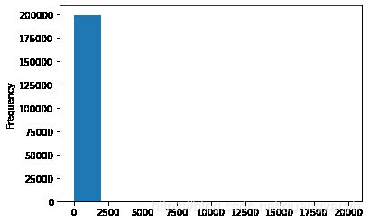
# 刚刚已经对 train 进行异常值处理了,但是还有这么奇怪的分布是因为 test 中的 power 异常值,
# 所以刚刚 train 中的 power 异常值不删为好,可以用长尾分布截断来代替
train['power'].plot.hist()
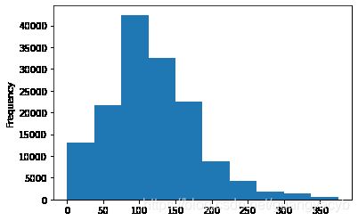
# 我们对其取 log,在做归一化
from sklearn import preprocessing
min_max_scaler = preprocessing.MinMaxScaler()
data['power'] = np.log(data['power'] + 1)
data['power'] = ((data['power'] - np.min(data['power'])) / (np.max(data['power']) - np.min(data['power'])))
data['power'].plot.hist()

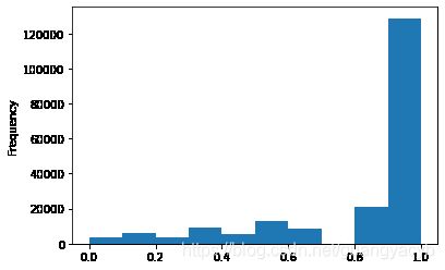
# km 的比较正常,应该是已经做过分桶了
data['kilometer'].plot.hist()

# 所以可以直接做归一化
data['kilometer'] = ((data['kilometer'] - np.min(data['kilometer'])) /
                        (np.max(data['kilometer']) - np.min(data['kilometer'])))
data['kilometer'].plot.hist()
# 除此之外 还有刚刚构造的统计量特征:
# 'brand_amount', 'brand_price_average', 'brand_price_max',
# 'brand_price_median', 'brand_price_min', 'brand_price_std',
# 'brand_price_sum'
# 这里不再一一举例分析,直接做变换,
def max_min(x):
    return (x - np.min(x)) / (np.max(x) - np.min(x))

data['brand_amount'] = ((data['brand_amount'] - np.min(data['brand_amount'])) /
                        (np.max(data['brand_amount']) - np.min(data['brand_amount'])))
data['brand_price_average'] = ((data['brand_price_average'] - np.min(data['brand_price_average'])) /
                               (np.max(data['brand_price_average']) - np.min(data['brand_price_average'])))
data['brand_price_max'] = ((data['brand_price_max'] - np.min(data['brand_price_max'])) /
                           (np.max(data['brand_price_max']) - np.min(data['brand_price_max'])))
data['brand_price_median'] = ((data['brand_price_median'] - np.min(data['brand_price_median'])) /
                              (np.max(data['brand_price_median']) - np.min(data['brand_price_median'])))
data['brand_price_min'] = ((data['brand_price_min'] - np.min(data['brand_price_min'])) /
                           (np.max(data['brand_price_min']) - np.min(data['brand_price_min'])))
data['brand_price_std'] = ((data['brand_price_std'] - np.min(data['brand_price_std'])) /
                           (np.max(data['brand_price_std']) - np.min(data['brand_price_std'])))
data['brand_price_sum'] = ((data['brand_price_sum'] - np.min(data['brand_price_sum'])) /
                           (np.max(data['brand_price_sum']) - np.min(data['brand_price_sum'])))
# 对类别特征进行 OneEncoder
data = pd.get_dummies(data, columns=['model', 'brand', 'bodyType', 'fuelType',
                                     'gearbox', 'notRepairedDamage', 'power_bin'])
print(data.shape)
data.columns
(199037, 370)


Index(['SaleID', 'name', 'power', 'kilometer', 'seller', 'offerType', 'price',
       'v_0', 'v_1', 'v_2',
       ...
       'power_bin_20.0', 'power_bin_21.0', 'power_bin_22.0', 'power_bin_23.0',
       'power_bin_24.0', 'power_bin_25.0', 'power_bin_26.0', 'power_bin_27.0',
       'power_bin_28.0', 'power_bin_29.0'],
      dtype='object', length=370)
# 这份数据可以给 LR 用
data.to_csv('data_for_lr.csv', index=0)
特征筛选
过滤式
# 相关性分析
print(data['power'].corr(data['price'], method='spearman'))
print(data['kilometer'].corr(data['price'], method='spearman'))
print(data['brand_amount'].corr(data['price'], method='spearman'))
print(data['brand_price_average'].corr(data['price'], method='spearman'))
print(data['brand_price_max'].corr(data['price'], method='spearman'))
print(data['brand_price_median'].corr(data['price'], method='spearman'))
0.5728285196051496
-0.4082569701616764
0.058156610025581514
0.3834909576057687
0.259066833880992
0.38691042393409447
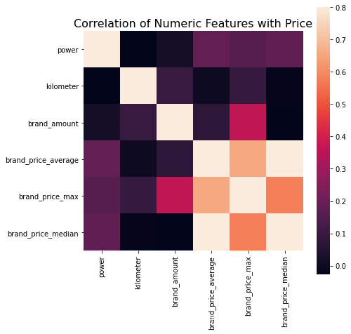
# 也可以直接看图
data_numeric = data[['power', 'kilometer', 'brand_amount', 'brand_price_average',
                     'brand_price_max', 'brand_price_median']]
correlation = data_numeric.corr()

f , ax = plt.subplots(figsize = (7, 7))
plt.title('Correlation of Numeric Features with Price',y=1,size=16)
sns.heatmap(correlation,square = True,  vmax=0.8)
包裹式
!pip install mlxtend
Collecting mlxtend
  Downloading mlxtend-0.17.2-py2.py3-none-any.whl (1.3 MB)
Requirement already satisfied: scipy>=1.2.1 in c:\anaconda3\envs\mytf\lib\site-packages (from mlxtend) (1.4.1)
Requirement already satisfied: setuptools in c:\anaconda3\envs\mytf\lib\site-packages (from mlxtend) (46.0.0.post20200311)
Requirement already satisfied: matplotlib>=3.0.0 in c:\anaconda3\envs\mytf\lib\site-packages (from mlxtend) (3.2.0)
Requirement already satisfied: scikit-learn>=0.20.3 in c:\anaconda3\envs\mytf\lib\site-packages (from mlxtend) (0.22.2.post1)
Requirement already satisfied: pandas>=0.24.2 in c:\anaconda3\envs\mytf\lib\site-packages (from mlxtend) (1.0.2)
Requirement already satisfied: numpy>=1.16.2 in c:\anaconda3\envs\mytf\lib\site-packages (from mlxtend) (1.18.1)
Requirement already satisfied: joblib>=0.13.2 in c:\anaconda3\envs\mytf\lib\site-packages (from mlxtend) (0.14.1)
Requirement already satisfied: cycler>=0.10 in c:\anaconda3\envs\mytf\lib\site-packages (from matplotlib>=3.0.0->mlxtend) (0.10.0)
Requirement already satisfied: kiwisolver>=1.0.1 in c:\anaconda3\envs\mytf\lib\site-packages (from matplotlib>=3.0.0->mlxtend) (1.1.0)
Requirement already satisfied: python-dateutil>=2.1 in c:\anaconda3\envs\mytf\lib\site-packages (from matplotlib>=3.0.0->mlxtend) (2.8.1)
Requirement already satisfied: pyparsing!=2.0.4,!=2.1.2,!=2.1.6,>=2.0.1 in c:\anaconda3\envs\mytf\lib\site-packages (from matplotlib>=3.0.0->mlxtend) (2.4.6)
Requirement already satisfied: pytz>=2017.2 in c:\anaconda3\envs\mytf\lib\site-packages (from pandas>=0.24.2->mlxtend) (2019.3)
Requirement already satisfied: six in c:\anaconda3\envs\mytf\lib\site-packages (from cycler>=0.10->matplotlib>=3.0.0->mlxtend) (1.14.0)
Installing collected packages: mlxtend
Successfully installed mlxtend-0.17.2
from mlxtend.feature_selection import SequentialFeatureSelector as SFS
from sklearn.linear_model import LinearRegression
sfs = SFS(LinearRegression(),
           k_features=10,
           forward=True,
           floating=False,
           scoring = 'r2',
           cv = 0)
x = data.drop(['price'], axis=1)
x = x.fillna(0)
y = data['price']
sfs.fit(x, y)
sfs.k_feature_names_

嵌入式
Lasso 回归和决策树可以完成嵌入式特征选择
大部分情况下都是用嵌入式做特征筛选
总结
- 模型在比赛中发挥的作用有时不如特征工程重要,没有好的特征再好的模型也发挥不了作用。
- 特征工程是为了从数据中提取出与问题目标相关联的信息,提高机器学习的性能。
- 特征构造有助于发掘原始数据没有直接给出的信息。
- 匿名特征往往不清楚特征相互直接的关联性,只有单纯基于特征进行处理:装箱,groupby,agg 等特征统计,还可以对特征进行的 log,exp 等变换,或者对多个特征进行四则运算(如上面算出的使用时长),多项式组合等然后进行筛选。
- 特性的匿名性限制了很多对于特征的处理,有些时候用 NN 去提取一些特征也会达到意想不到的良好效果。
- 若知道特征含义,可以基于信号处理,频域提取,丰度,偏度等构建更为有实际意义的特征,如在推荐系统中,各种类型点击率统计,各时段统计,加用户属性的统计等等,这种特征构建往往要深入分析背后的业务逻辑,才能更好的找到 magic。
- 特征工程往往与模型密切结合,所以要为 LR NN 做分桶和特征归一化,对于特征的处理效果和特征重要性等往往要通过模型来验证。