机器学习入门之逻辑回归(2)- 微芯片质量预测-非线性(python实现)
一、基础知识
- 我们先看一下数据集的点的分布图像:
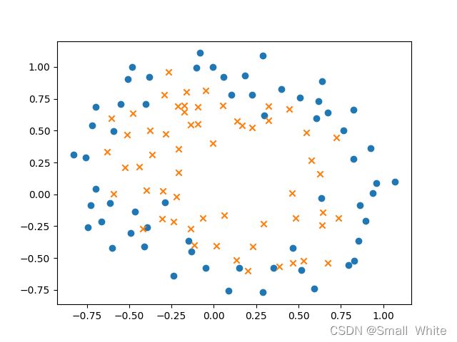
从上述图像中我们不能得到线性的方程,拟合上面的图像,显然不能用常规的图形去表示它,所以我们要用非线性的函数去拟合它。 - 如果我们只用两个特征去拟合它,只会得到一个线性的分界线,在逻辑回归的第一篇博文中是两个特征拟合出来的边界。如果我们需要拟合出来一个非线性的曲线,那么就需要升维,也就是将只有 x 1 、 x 2 x_1、x_2 x1、x2的项升维到 x 1 , x 2 , x 1 2 , x 1 x 2 , x 2 2 , ⋯ , x i n x_1,x_2,x_1^2,x_1x_2,x_2^2,\cdots,x_i^n x1,x2,x12,x1x2,x22,⋯,xin,本篇案例中升维到了 x i 6 x_i^6 xi6,升维后就到了28个特征,此时我们会得到非线性的边界,但是,为了消除高阶对拟合的影响,即防止出现过拟合线性,我们要对其损失函数进行正则化,正则化的方式在线性回归系列文章中的
波士顿房价预测中有讲解,逻辑回归与线性回归的正则化方式是相同的。
下面介绍一下升维的python代码:
def new_featuremeth(x1,x2):
    new_feature = np.ones((int(np.size(x1)),1))
    index = 1
    for i in range(1,7):
        for j in range(i+1):
            new_feature =  np.insert(new_feature,index,np.power(x1,(i-j))*np.power(x2,j),axis=1)
            index+=1
    return new_feature
接下来设的目标函数的参数 θ j \theta_j θj也应该是对应的28个。
3. 逻辑回归正则化
对于逻辑回归的正则化,方式与线性回归相同,在损失函数中加入正则化项,同时在梯度函数中加入求导后的正则化项。
加上正则化的损失函数:
J ( θ ) = 1 m ( ∑ i = 1 m ( − y ( i ) l n ( h θ ( x ( i ) ) ) − ( 1 − y ( i ) ) l n ( 1 − h θ ( x ( i ) ) ) ) ) + λ 2 m ∑ j = 1 n θ j 2 J(\theta) = \frac{1}{m}(\sum_{i = 1}^{m}(-y^{(i)}ln(h_\theta(x^{(i)}))-(1-y^{(i)})ln(1-h_\theta(x^{(i)})))) + \frac{\lambda}{2m}\sum_{j=1}^{n}\theta_j^2 J(θ)=m1(i=1∑m(−y(i)ln(hθ(x(i)))−(1−y(i))ln(1−hθ(x(i)))))+2mλj=1∑nθj2
加上正则化的梯度函数:
θ 0 : = θ 0 − 1 m ( ∑ i = 1 m ( h θ ( x ( i ) ) − y ( i ) ) x j ) j = 0 \theta_0 := \theta_0-\frac{1}{m}(\sum_{i=1}^{m}(h_\theta(x^{(i)})-y^{(i)})x_j) \ \ \ \ \ \ \ \ \ \ j = 0 θ0:=θ0−m1(i=1∑m(hθ(x(i))−y(i))xj) j=0
θ j : = θ j − 1 m ( ∑ i = 1 m ( h θ ( x ( i ) ) − y ( i ) ) x j ) + λ m θ j j > 0 \theta_j := \theta_j - \frac{1}{m}(\sum_{i=1}^{m}(h_\theta(x^{(i)})-y^{(i)})x_j) + \frac{\lambda}{m}\theta_j \ \ \ \ \ \ \ \ j>0 θj:=θj−m1(i=1∑m(hθ(x(i))−y(i))xj)+mλθj j>0
4. 由于逻辑回归的 λ \lambda λ 和 α \alpha α 不容易确定,所以我们使用高级优化方式,具体介绍在上一篇的逻辑回归中有讲解。
二、代码实现
- 读取与处理数据、拟合图、误差图代码,文件名:
logisticnolinerregress.py
from cmath import cos
from hashlib import new
from math import ceil
import scipy.optimize as opt
from operator import lt
import numpy as np
import matplotlib.pyplot as plt
from pyparsing import Opt, re
origi_data = np.loadtxt('ex2data2.txt',delimiter=',')
theta = np.arange(start=0.1,stop=2.9,step=0.1)
lamdba = 0.5
origi_data_zero = origi_data[origi_data[:,2]==0]
origi_data_one = origi_data[origi_data[:,2]==1]
origi_data_zero_x1 = origi_data_zero[:,0]
origi_data_zero_x2 = origi_data_zero[:,1]
origi_data_one_x1 = origi_data_one[:,0]
origi_data_one_x2 = origi_data_one[:,1]
print(np.size(origi_data))
test_data = origi_data[-ceil(0.2*origi_data.shape[0]):,:]
origi_data = origi_data[0:int(0.8*origi_data.shape[0]),:]
print(np.size(test_data))
print(np.size(origi_data))
origin_data_y = origi_data[:,-1]
# 添加特征
origi_data_x1 = origi_data[:,0]
origi_data_x2 = origi_data[:,1]
error_array = np.array([])
def new_featuremeth(x1,x2):
new_feature = np.ones((int(np.size(x1)),1))
index = 1
for i in range(1,7):
for j in range(i+1):
# print('x1^{},x2^{}'.format((i-j),j))
new_feature = np.insert(new_feature,index,np.power(x1,(i-j))*np.power(x2,j),axis=1)
# print(new_feature)
index+=1
return new_feature
def cost(theta,x,y,lamdba):
global error_array
theta_x = np.dot(theta,x.T)
error_y = sigmoid(theta_x)
cost_error = ((np.dot(y,np.log(error_y).T)+ np.dot((1-y),np.log(1-error_y).T))/(-np.size(y)))+((lamdba*np.dot(theta[1:],theta[1:].T))/(2*np.size(y)))
error_array = np.concatenate((error_array,[cost_error]),axis=0)
return cost_error
def sigmoid(z):
return 1/( 1 + np.exp(-z))
def gredient(theta,x,y,lamdba):
# lamdba = 25
theta_x = np.dot(theta,x.T)
error_cost_y = sigmoid(theta_x)-y
gradient_array = np.array([np.sum(error_cost_y)/np.size(y)])
gredient_error = (np.dot(error_cost_y,x[:,1:])+lamdba*theta[1:])/np.size(y)
gradient_array = np.concatenate((gradient_array,gredient_error),axis=0)
print('下降函数{}'.format(gradient_array))
return gradient_array
# result = opt.fmin_tnc(func=cost,x0=theta,fprime=gredient,args=(new_feature,origin_data_y))
new_feature = new_featuremeth(origi_data_x1,origi_data_x2)
result = opt.minimize(fun=cost, args=(new_feature,origin_data_y,lamdba), jac=gredient, x0=theta, method='TNC')
print(result)
theta = result['x']
print(theta)
x_axis = np.arange(np.size(error_array)).reshape(np.size(error_array),1)
# print(error_array)
plt.plot(x_axis,error_array)
plt.show()
u = np.linspace(-1, 1.5, 50);
v = np.linspace(-1, 1.5, 50);
# print(u)
z = np.zeros((np.size(u), np.size(v)));
for i in range(1,np.size(u)):
for j in range(1,np.size(v)):
# print(new_featuremeth(u[i], v[j]))
z[i][j] =np.dot(theta,new_featuremeth(u[i], v[j]).T)
plt.scatter(origi_data_zero_x1,origi_data_zero_x2,marker='o')
plt.scatter(origi_data_one_x1,origi_data_one_x2,marker='x')
# 此处需要转置,因为x2是纵坐标,所以对应的是z的列,但是循环生成的时候是按照行添加的,所以需要转置
z = z.T
plt.contour(u,v,z,[0])
plt.show()
#测试集
test_data_x = test_data[:,:2]
test_data_y = test_data[:,-1]
new_feature_test = new_featuremeth(test_data_x[:,0],test_data_x[:,1])
theta_x = np.dot(theta,new_feature_test.T)
error_cost_y = sigmoid(theta_x)
count = 0
for i in range(np.size(error_cost_y)):
if error_cost_y[i]>0.5:
if test_data_y[i]==1:
count+=1
if error_cost_y[i]<=0.5:
if test_data_y[i]==0:
count+=1
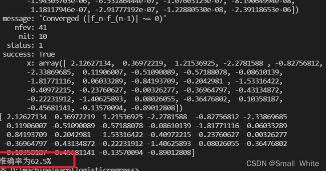
print('准确率为{}%'.format((count/np.size(test_data_y))*100))
- 则我们可以得到下面的拟合图与优化过程图
下面是拟合的边界曲线:

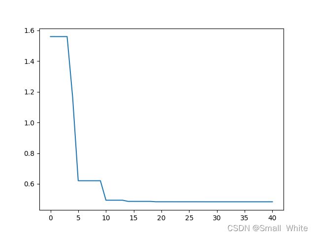
下面是优化图像:
下面是准确率:
三、样本集
复制放进txt中即可
0.051267,0.69956,1
-0.092742,0.68494,1
-0.21371,0.69225,1
-0.375,0.50219,1
-0.51325,0.46564,1
-0.52477,0.2098,1
-0.39804,0.034357,1
-0.30588,-0.19225,1
0.016705,-0.40424,1
0.13191,-0.51389,1
0.38537,-0.56506,1
0.52938,-0.5212,1
0.63882,-0.24342,1
0.73675,-0.18494,1
0.54666,0.48757,1
0.322,0.5826,1
0.16647,0.53874,1
-0.046659,0.81652,1
-0.17339,0.69956,1
-0.47869,0.63377,1
-0.60541,0.59722,1
-0.62846,0.33406,1
-0.59389,0.005117,1
-0.42108,-0.27266,1
-0.11578,-0.39693,1
0.20104,-0.60161,1
0.46601,-0.53582,1
0.67339,-0.53582,1
-0.13882,0.54605,1
-0.29435,0.77997,1
-0.26555,0.96272,1
-0.16187,0.8019,1
-0.17339,0.64839,1
-0.28283,0.47295,1
-0.36348,0.31213,1
-0.30012,0.027047,1
-0.23675,-0.21418,1
-0.06394,-0.18494,1
0.062788,-0.16301,1
0.22984,-0.41155,1
0.2932,-0.2288,1
0.48329,-0.18494,1
0.64459,-0.14108,1
0.46025,0.012427,1
0.6273,0.15863,1
0.57546,0.26827,1
0.72523,0.44371,1
0.22408,0.52412,1
0.44297,0.67032,1
0.322,0.69225,1
0.13767,0.57529,1
-0.0063364,0.39985,1
-0.092742,0.55336,1
-0.20795,0.35599,1
-0.20795,0.17325,1
-0.43836,0.21711,1
-0.21947,-0.016813,1
-0.13882,-0.27266,1
0.18376,0.93348,0
0.22408,0.77997,0
0.29896,0.61915,0
0.50634,0.75804,0
0.61578,0.7288,0
0.60426,0.59722,0
0.76555,0.50219,0
0.92684,0.3633,0
0.82316,0.27558,0
0.96141,0.085526,0
0.93836,0.012427,0
0.86348,-0.082602,0
0.89804,-0.20687,0
0.85196,-0.36769,0
0.82892,-0.5212,0
0.79435,-0.55775,0
0.59274,-0.7405,0
0.51786,-0.5943,0
0.46601,-0.41886,0
0.35081,-0.57968,0
0.28744,-0.76974,0
0.085829,-0.75512,0
0.14919,-0.57968,0
-0.13306,-0.4481,0
-0.40956,-0.41155,0
-0.39228,-0.25804,0
-0.74366,-0.25804,0
-0.69758,0.041667,0
-0.75518,0.2902,0
-0.69758,0.68494,0
-0.4038,0.70687,0
-0.38076,0.91886,0
-0.50749,0.90424,0
-0.54781,0.70687,0
0.10311,0.77997,0
0.057028,0.91886,0
-0.10426,0.99196,0
-0.081221,1.1089,0
0.28744,1.087,0
0.39689,0.82383,0
0.63882,0.88962,0
0.82316,0.66301,0
0.67339,0.64108,0
1.0709,0.10015,0
-0.046659,-0.57968,0
-0.23675,-0.63816,0
-0.15035,-0.36769,0
-0.49021,-0.3019,0
-0.46717,-0.13377,0
-0.28859,-0.060673,0
-0.61118,-0.067982,0
-0.66302,-0.21418,0
-0.59965,-0.41886,0
-0.72638,-0.082602,0
-0.83007,0.31213,0
-0.72062,0.53874,0
-0.59389,0.49488,0
-0.48445,0.99927,0
-0.0063364,0.99927,0
0.63265,-0.030612,0
以上若有问题,请大佬指出,感激不尽,共同进步。