Matlab:拟合(2)

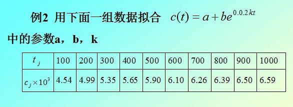
非线性最小二乘拟合：

解法一：用命令lsqcurvefit

1 function f = curvefun(x, tdata)

2 f = x(1) + x(2)*exp(0.02 * x(3) * tdata);

3 %其中x(1) = a; x(2) = b; x(3) = c;

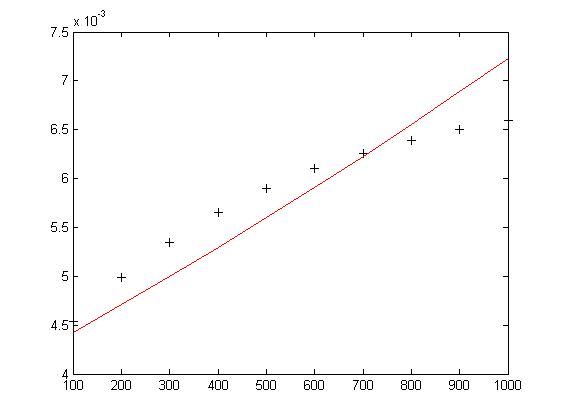
 1 %数据输入

 2 tdata = 100:100:1000;

 3 cdata = 1e-03 * [4.54, 4.99, 5.35, 5.65, 5.90, 6.10, 6.26, 6.39, 6.50, 6.59];

 4 %设定预测值

 5 x0 = [0.2 0.05 0.05];

 6 %非线性拟合函数

 7 x = lsqcurvefit('curvefun', x0, tdata, cdata)

 8 %作图

 9 f = curvefun(x, tdata)

10 plot(tdata, cdata, 'k+')

11 hold on

12 plot(tdata, f, 'r')

结果：
x =

   -0.0074    0.0116    0.0118

f =

  Columns 1 through 8

    0.0044    0.0047    0.0050    0.0053    0.0056    0.0059    0.0062    0.0066

  Columns 9 through 10

    0.0069    0.0072

解法二：用命令lsqnonlin

1 function f = curvefun1(x)

2 %curvefun1的自变量是x，cdata和tdata是已知参数，故应将cdata,tdata的值卸载curvefun1中

3 tdata = 100:100:1000;

4 cdata = 1e-03 * [4.54, 4.99, 5.35, 5.65, 5.90, 6.10, 6.26, 6.39, 6.50, 6.59];

5 f = x(1) + x(2)*exp(0.02 * x(3) * tdata) - cdata;%注意

1 tdata = 100:100:1000;

2 cdata = 1e-03 * [4.54, 4.99, 5.35, 5.65, 5.90, 6.10, 6.26, 6.39, 6.50, 6.59];

3 %预测值

4 x0 = [0.2 0.05 0.05];

5 x = lsqnonlin('curvefun1', x0)

6 f = curvefun1(x)

7 plot(tdata, cdata, 'k+')

8 hold on

9 plot(tdata, f+cdata, 'r')

结果：

x =

   -0.0074    0.0116    0.0118

f =

  1.0e-003 *

  Columns 1 through 8

   -0.1168   -0.2835   -0.3534   -0.3564   -0.3022   -0.1908   -0.0320    0.1645

  Columns 9 through 10

    0.3888    0.6411