在Azure ML中使用Logistic回归预测客户的贷款资格
This article aims to provide the basics of creating Logistic Regression in Azure ML by designing a simple model step-by-step.
本文旨在通过逐步设计一个简单的模型,提供在Azure ML中创建Logistic回归的基础。
Predicting whether or not a customer is eligible for a loan is a very important problem for banks and other financial institutes. Ideally, a loan should only be approved for those customers who are likely to pay the money back, and should not be approved for the customers that are likely to default.
对于银行和其他金融机构而言,预测客户是否有资格获得贷款是一个非常重要的问题。 理想情况下,贷款应仅批准给可能还钱的客户,而不应批准给可能违约的客户。
Fortunately, if we have sufficient data, we can use statistical algorithms to develop a model that can successfully predict whether a loan should be approved for the customers or not. One such algorithm is the logistic regression algorithm. In this article, we will see how to create a logistic regression in Azure ML Studio that can predict customer’s loan eligibility.
幸运的是,如果我们有足够的数据,则可以使用统计算法来开发一个模型,该模型可以成功地预测是否应为客户批准贷款。 一种这样的算法是逻辑回归算法。 在本文中,我们将看到如何在Azure ML Studio中创建逻辑回归,该回归可以预测客户的贷款资格。
数据集 (The Dataset)
The dataset for this problem can be downloaded freely from this Kaggle Link. The data will be downloaded in a compressed file. If you extract the compressed file, you will see two files: “train_u6lujuX_CVtuZ9i.csv” and “test_Y3wMUE5_7gLdaTN.csv”. We will be working with the “train_u6lujuX_CVtuZ9i.csv” file. You can simply rename it to “train_loan.csv”.
可以从Kaggle Link免费下载该问题的数据集。 数据将以压缩文件下载。 如果解压缩文件,将看到两个文件:“ train_u6lujuX_CVtuZ9i.csv”和“ test_Y3wMUE5_7gLdaTN.csv”。 我们将使用“ train_u6lujuX_CVtuZ9i.csv”文件。 您可以将其重命名为“ train_loan.csv”。
The next step is to upload the file to the Azure ML Studio. Login to Azure ML Studio account and go to this link: https://studio.azureml.net/Home/.
下一步是将文件上传到Azure ML Studio。 登录到Azure ML Studio帐户,然后转到此链接: https : //studio.azureml.net/Home/ 。
To upload the dataset, click on the “DATASETS” option from the menu on the left and then click the “+NEW” button at the bottom right of the screen as shown below:
要上传数据集,请单击左侧菜单中的“ DATASETS”选项,然后单击屏幕右下方的“ + NEW”按钮,如下所示:
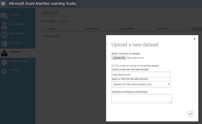
You will see a file upload dialogue box. Click the “FROM LOCAL FILE” and then “Choose File” option to upload a file from your drive. In my case, I renamed the file “train_u6lujuX_CVtuZ9i.csv” to “train_loan.csv” and uploaded it. Look at the following screenshot for reference:
您将看到一个文件上传对话框。 单击“从本地文件”,然后单击“选择文件”选项以从驱动器上载文件。 就我而言,我将文件“ train_u6lujuX_CVtuZ9i.csv”重命名为“ train_loan.csv”并上传了文件。 请看以下屏幕截图以供参考:
Wait a few seconds for the dataset to upload. Once the dataset is uploaded, you should see the uploaded dataset in the list of datasets as shown below:
等待几秒钟,以便数据集上载。 数据集上传后,您应该在数据集列表中看到上传的数据集,如下所示:
创建简单的贷款资格预测模型 (Creating a Simple Prediction Model for Loan Eligibility Prediction)
In this section, we will create a simple logistic regression in the Azure ML model that will be trained using the dataset that we uploaded in the previous section and will be used to make predictions about whether a bank should award a loan to a customer or not.
在本节中,我们将在Azure ML模型中创建一个简单的逻辑回归,该回归将使用上一节中上传的数据集进行训练,并将用于预测银行是否应向客户提供贷款。
Follow these steps:
跟着这些步骤:
创建一个新实验 (Creating a New Experiment)
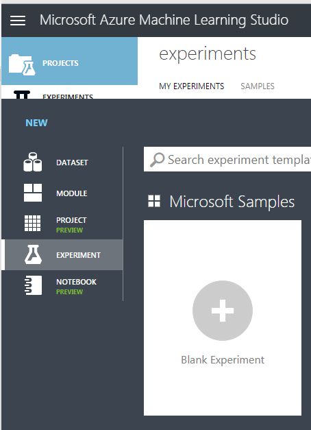
To create a new experiment the “EXPERIMENTS” option from the Azure ML Studio dashboard. You will be presented with different types of options. Select “Blank Experiment” as shown below:
若要创建新实验,请从Azure ML Studio仪表板中选择“ EXPERIMENTS”选项。 您将看到不同类型的选项。 选择“空白实验”,如下所示:
You will be presented with a new experiment dashboard.
您将看到一个新的实验仪表板。
向实验添加数据集 (Adding a Dataset to the Experiment)
The first step to creating a logistic regression in Azure ML is to add the dataset to the experiment dashboard. We will add the “train_loan.csv” dataset to the experiment. To do so, click on “Saved Datasets -> My Datasets” and then drag the “train_loan.csv” file to the experiment dashboard. Look at the following screenshot for reference.
在Azure ML中创建逻辑回归的第一步是将数据集添加到实验仪表板。 我们将“ train_loan.csv”数据集添加到实验中。 为此,请单击“保存的数据集->我的数据集”,然后将“ train_loan.csv”文件拖到实验仪表板上。 请看以下屏幕截图以供参考。
可视化数据 (Visualizing the Data)
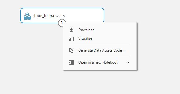
Let’s visualize our dataset. Right-click on the circle node containing digit 1 from the dataset module. From the drop-down list, select “Visualize” as shown below:
让我们可视化我们的数据集。 右键单击数据集模块中包含数字1的圆节点。 从下拉列表中选择“ Visualize”,如下所示:
If you visualize the dataset, you will see that the data has 614 rows and 13 columns. The last column is the “Loan_Status” column. As I earlier said, this is a supervised learning problem, therefore in the training data we already have the true or real outputs. Our model will learn how to predict whether a customer is eligible for the loan or not using the data in the first 12 columns.
如果可视化数据集,您将看到数据具有614行和13列。 最后一列是“ Loan_Status”列。 就像我之前说的,这是一个监督学习问题,因此在训练数据中我们已经有了真实或真实的输出。 我们的模型将使用前12列中的数据学习如何预测客户是否有资格获得贷款。
处理缺失值 (Handling Missing Values)
Before we can learn from the data or in other words, train our model on the data, we have to handle the missing values. To check the missing values in each column, simply click the column header. For instance, if you click the column “Married”, you will see that 3 values are missing as shown below:
在我们可以从数据中学习或换句话说,在数据上训练我们的模型之前,我们必须处理缺失的值。 要检查每列中的缺失值,只需单击列标题。 例如,如果单击“已婚”列,您将看到缺少3个值,如下所示:
If you visualize all the columns for missing values, you will see that among categorical columns, Gender, Married, Dependents, Self_Employed, and Credit_History columns contain missing values. The Credit_History column contains two unique values 1 and 0, therefore we can treat it as a categorical column. The rest of the categorical columns contain data in the form of string.
如果可视化所有列以查找缺失值,则将在分类列中看到“性别”,“已婚”,“受抚养者”,“自雇型”和“贷方历史”列包含缺失值。 Credit_History列包含两个唯一值1和0,因此我们可以将其视为分类列。 其余分类列包含字符串形式的数据。
To handle missing data for categorical columns, we will use the “Clean Missing Data” module. To do so, go to “Data Transformations -> Manipulations” and drag the “Clean Missing Data” module to the experiment dashboard. Connect the dataset module with the “Clean Missing Data” module as shown below:
要处理分类列的缺失数据,我们将使用“清除缺失数据”模块。 为此,请转到“数据转换->操作”,然后将“清除丢失的数据”模块拖到实验仪表板上。 如下所示,将数据集模块与“清除缺少的数据”模块连接:
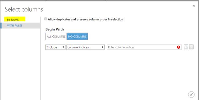
Next, click on the “Clean Missing Data” module. From the options in the right options bar, click “Launch Column Selector”. Select “NO COLUMNS” for the “Begin With” option. And then from the options on the left, select “BY NAME” as shown below:
接下来,单击“清除丢失的数据”模块。 在右侧选项栏中的选项中,单击“启动列选择器”。 为“开始于”选项选择“无栏”。 然后从左侧的选项中选择“ BY NAME”,如下所示:
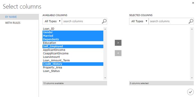
Next, we need to select the Gender, Married, Dependents, Self_Employed and Credit_History columns and add them to the list of SELECTED columns. The following screenshot is for reference:
接下来,我们需要选择“性别”,“已婚”,“受抚养者”,“自雇”和“信用历史”列,并将它们添加到“选择”列的列表中。 以下屏幕截图仅供参考:
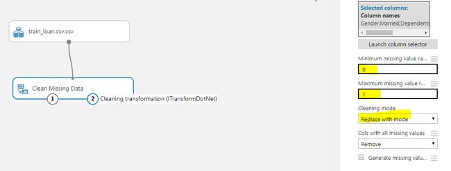
Now, set the “Minimum missing value ratio” to 0 and “Maximum missing value ratio” to 1. This means that we want to replace all the missing values. From the “Cleaning mode” dropdown list. Select “Replace with mode” which means that we want to replace missing values with the most frequently occurring values in the corresponding columns. Look at the highlighted values in the following screenshot, for reference.
现在,将“最小缺失值比率”设置为0,将“最大缺失值比率”设置为1。这意味着我们要替换所有缺失值。 从“清洁模式”下拉列表中。 选择“用模式替换”,这意味着我们要用相应列中最频繁出现的值替换缺失的值。 查看以下屏幕快照中突出显示的值,以供参考。
Finally, to clean the data, simply right click on the “Clean Missing Data” module and then select “Run Selected”. The missing values in the categorical columns will be replaced with the most frequently occurring values. Now is the time to handle missing values in the numerical columns.
最后,要清理数据,只需右键单击“清理丢失的数据”模块,然后选择“运行选定项”。 类别列中的缺失值将替换为最常出现的值。 现在是时候处理数字列中的缺失值了。
Among numerical columns in our dataset, LoanAmount and Loan_Amount_Term contain missing values. The process to handle these values is the same. Add a new “Clean Missing Data” module, launch the column selector and then select the LoanAmount and Loan_Amount_Term columns. Set the “Minimum missing value ratio” to 0 and “Maximum missing value ratio” to 1. Since, we are now dealing with numeric data, for the “Cleaning mode” we will select the value “Replace with mean” which will replace all the missing numerical values with the mean of the rest of the column values.
在我们的数据集中的数字列中,LoanAmount和Loan_Amount_Term包含缺失值。 处理这些值的过程是相同的。 添加一个新的“清除缺少的数据”模块,启动列选择器,然后选择LoanAmount和Loan_Amount_Term列。 将“最小缺失值比率”设置为0,将“最大缺失值比率”设置为1。由于我们现在正在处理数字数据,因此对于“清洁模式”,我们将选择值“用均值替换”,它将替换所有缺少的数值以及其余列值的平均值。
选择列 (Selecting Columns)
Selecting columns or features is an area of research in itself. However, our problem will select all the columns in our dataset except the “Loan_ID.” Since the LOAN_ID has no impact on whether or not a customer is eligible for loan or not. To select columns, you can use the “Select Columns in Dataset” module which can be found inside “Data Transformation -> Manipulation”. The “Launch column selector” can be used to select columns as we did on in the last section. Finally, right-click on the “Select Columns in Dataset” module and then select “Run Selected”.
选择列或特征本身就是研究的领域。 但是,我们的问题将选择数据集中除“ Loan_ID”之外的所有列。 由于LOAN_ID对客户是否有资格获得贷款没有影响。 要选择列,可以使用“数据集中的选择列”模块,该模块可在“数据转换->操作”中找到。 如上一节所述,“启动列选择器”可用于选择列。 最后,右键单击“在数据集中选择列”模块,然后选择“运行选定项”。
在训练和测试集中拆分数据 (Splitting Data in Training and Testing Set)
We are dealing with a supervised learning problem where the algorithm learns from ground truth and is evaluated on new unseen values. We will divide our data into two sets: Training and Testing set. Our logistic regression in Azure ML will be trained on the training data (will learn to predict customer’s loan eligibility from the training data). After we train the algorithm, we will evaluate how well our algorithm performs, using the test data.
我们正在处理一个监督学习问题,其中该算法从地面真理中学习,并根据新的看不见的值进行评估。 我们将数据分为两组:训练组和测试组。 我们将在训练数据上训练我们在Azure ML中的逻辑回归(将通过训练数据学习预测客户的贷款资格)。 训练算法后,我们将使用测试数据评估算法的性能。
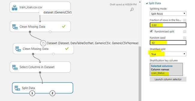
To split the data, we can use the “Split Data” module from “Data Transformations -> Sample and Split”. We need to specify a few parameters for the “Split” data module. From the options on the right of the dashboard, set the value of “Fractions of rows in the first output dataset” to 0.80, which means that 0.80 of the data will be used for training the algorithm. For random seed, you can specify any value. I specified 42. Finally, set “Stratified split” to true. The stratified split equally divides our data with respect to specific columns. We will specify “Loan_Status” as the column for a stratified split using the column selector. Look at the following screenshot for reference:
要拆分数据,我们可以使用“数据转换->采样和拆分”中的“拆分数据”模块。 我们需要为“拆分”数据模块指定一些参数。 从仪表板右侧的选项中,将“第一个输出数据集中的行的分数”的值设置为0.80,这意味着将使用0.80的数据来训练算法。 对于随机种子,可以指定任何值。 我指定了42。最后,将“分层拆分”设置为true。 分层拆分将我们的数据相对于特定列平均划分。 我们将使用列选择器将“ Loan_Status”指定为分层拆分的列。 请看以下屏幕截图以供参考:
As the last step, right-click on the “Split Data” module and then select “Run Selected”.
作为最后一步,右键单击“拆分数据”模块,然后选择“运行所选内容”。
在Azure ML算法中训练逻辑回归 (Training the Logistic Regression in Azure ML Algorithm)
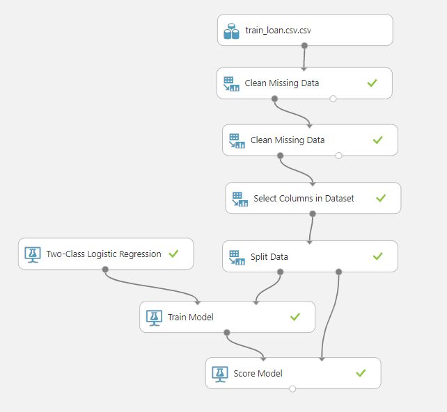
To train the logistic regression in Azure ML, we can use the “Two-Class Logistic Regression Module” which is available inside the “Machine Learning” module. Next, we need to import the “Train Model” module from the “Machine Learning -> Train”. We need to provide the output of the “Split Data” module and the “Two-Class Logistic Regression Module”, as input to the “Train Model” module. Furthermore, using the column selector for the “Train Model” module, you need to select the column that you want to predict. In our case we need to predict “Loan_Status”, therefore we select this column.
若要在Azure ML中训练逻辑回归,我们可以使用“机器学习”模块中提供的“两类逻辑回归模块”。 接下来,我们需要从“机器学习->火车”中导入“火车模型”模块。 我们需要提供“拆分数据”模块和“两类逻辑回归模块”的输出,作为“培训模型”模块的输入。 此外,将列选择器用于“训练模型”模块,您需要选择要预测的列。 在我们的情况下,我们需要预测“ Loan_Status”,因此我们选择此列。
Lastly, we need to add the “Score” module from the “Machine Learning -> Score” module which will find the score of each prediction made by our logistic regression in Azure ML. Look at the following screenshot.
最后,我们需要从“机器学习->得分”模块中添加“得分”模块,该模块将找到通过Azure ML中的逻辑回归做出的每个预测的得分。 看下面的截图。
Right-click on the “Score Model” module and then select “Run Selected”.
右键单击“得分模型”模块,然后选择“运行选定项”。
To visualize the score, right-click on the “Score model” node and select “Visualize”. You will see that to more columns i.e. “Scored Label” and “Scored Probabilities” have been added to the dataset as shown below:
要可视化分数,请右键单击“分数模型”节点,然后选择“可视化”。 您会看到,在更多列中,即“得分标签”和“得分概率”已添加到数据集中,如下所示:
The “Scored Label” contains the prediction and the “Scored Probabilities” contain the probability of prediction. For instance, from the first row, we can evaluate that the customer loan was approved as it is a Y in the “Scored Labels” column. The predicted probability that the loan was approved is 0.899.
“得分标签”包含预测,“得分概率”包含预测概率。 例如,在第一行中,我们可以评估“ Scored Labels”(评分标签)列中的客户贷款是否为Y。 贷款批准的预计概率为0.899。
在Azure ML算法中评估逻辑回归 (Evaluating the Logistic Regression in Azure ML Algorithm)
To evaluate the logistic regression in the Azure ML model, we can use the “Evaluate Model” submodule from the “Machine Learning” module. Connect the “Score Model” module with the “Evaluate Model” module. The full model looks like this:
要评估Azure ML模型中的逻辑回归,我们可以使用“机器学习”模块中的“评估模型”子模块。 将“得分模型”模块与“评估模型”模块连接。 完整的模型如下所示:
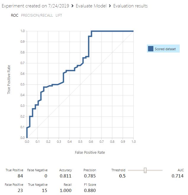
Finally, run the “Evaluate Model” module and then right-click it and click “Visualize” from the drop-down list. You should see the following results:
最后,运行“评估模型”模块,然后右键单击它,然后从下拉列表中单击“可视化”。 您应该看到以下结果:
Our model achieves an accuracy of 0.811 percent which means that 81% of the time, our model can correctly predict whether a customer is eligible for loans or not.
我们的模型达到0.811%的准确性,这意味着在81%的时间里,我们的模型可以正确地预测客户是否符合贷款条件。
结论 (Conclusion)
In this article, we saw how to create a simple logistic regression in Azure ML model to predict a customer’s eligibility for a bank loan, based on the features such as gender, marital status, employment, credit history etc. We saw how easy it is to create a prediction model in Azure ML Studio without writing a single line of code. Along the way, we discussed various steps to create a two-class logistic regression model for making predictions.
在本文中,我们了解了如何在Azure ML模型中基于性别,婚姻状况,就业,信用记录等功能,创建一个简单的逻辑回归来预测客户的银行贷款资格。我们看到了这是多么容易在Azure ML Studio中创建预测模型而无需编写任何代码。 在此过程中,我们讨论了创建两类逻辑回归模型以进行预测的各种步骤。
In case, you are interested in understanding integration of SQL Server and Azure ML, go over this article, Integrate SQL Server and Azure Machine Learning.
如果您有兴趣了解SQL Server和Azure ML的集成 ,请阅读本文“ 集成SQL Server和Azure机器学习” 。
本的其他精彩文章 (Other great articles from Ben)
| Understanding SQL Server case statement |
| Machine Learning Services – Configuring R Services in SQL Server |
| Importing and Working with CSV Files in SQL Server |
| 了解SQL Server的案例声明 |
| 机器学习服务–在SQL Server中配置R服务 |
| 在SQL Server中导入和使用CSV文件 |
翻译自: https://www.sqlshack.com/using-logistic-regression-in-azure-ml-for-predicting-customers-loan-eligibility/

