【智能优化算法-灰狼算法】基于狩猎 (DLH) 搜索策略的灰狼算法求解单目标优化问题附matlab代码
1 内容介绍
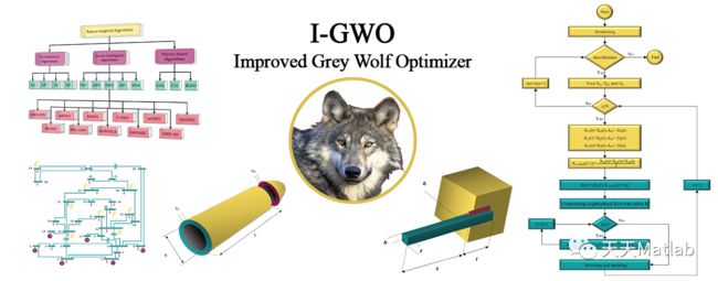
Grey wolf optimization (GWO) algorithm is a new emerging algorithm that is based on the social hierarchy of grey wolves as well as their hunting and cooperation strategies. Introduced in 2014, this algorithm has been used by a large number of researchers and designers, such that the number of citations to the original paper exceeded many other algorithms. In a recent study by Niu et al., one of the main drawbacks of this algorithm for optimizing real﹚orld problems was introduced. In summary, they showed that GWO's performance degrades as the optimal solution of the problem diverges from 0. In this paper, by introducing a straightforward modification to the original GWO algorithm, that is, neglecting its social hierarchy, the authors were able to largely eliminate this defect and open a new perspective for future use of this algorithm. The efficiency of the proposed method was validated by applying it to benchmark and real﹚orld engineering problems.
2 仿真代码
%___________________________________________________________________%
 %  Grey Wolf Optimizer (GWO) source codes version 1.0               %
 %                                                                   %
 %  Developed in MATLAB R2011b(7.13)                                 %
 %                                                                   %
 %  Author and programmer: Seyedali Mirjalili                        %
 %                                                                   %
 %         e-Mail: [email protected]                           %
 %                 [email protected]             %
 %                                                                   %
 %       Homepage: http://www.alimirjalili.com                       %
 %                                                                   %
 %   Main paper: S. Mirjalili, S. M. Mirjalili, A. Lewis             %
 %               Grey Wolf Optimizer, Advances in Engineering        %
 %               Software , in press,                                %
 %               DOI: 10.1016/j.advengsoft.2013.12.007               %
 %                                                                   %
 %___________________________________________________________________%
% This function containts full information and implementations of the benchmark
 % functions in Table 1, Table 2, and Table 3 in the paper
% lb is the lower bound: lb=[lb_1,lb_2,...,lb_d]
 % up is the uppper bound: ub=[ub_1,ub_2,...,ub_d]
 % dim is the number of variables (dimension of the problem)
function [lb,ub,dim,fobj] = Get_Functions_details(F)
switch F
     case 'F1'
         fobj = @F1;
         lb=-100;
         ub=100;
         dim=30;

     case 'F2'
         fobj = @F2;
         lb=-10;
         ub=10;
         dim=30;

     case 'F3'
         fobj = @F3;
         lb=-100;
         ub=100;
         dim=30;

     case 'F4'
         fobj = @F4;
         lb=-100;
         ub=100;
         dim=30;

     case 'F5'
         fobj = @F5;
         lb=-30;
         ub=30;
         dim=30;

     case 'F6'
         fobj = @F6;
         lb=-100;
         ub=100;
         dim=30;

     case 'F7'
         fobj = @F7;
         lb=-1.28;
         ub=1.28;
         dim=30;

     case 'F8'
         fobj = @F8;
         lb=-500;
         ub=500;
         dim=30;

     case 'F9'
         fobj = @F9;
         lb=-5.12;
         ub=5.12;
         dim=30;

     case 'F10'
         fobj = @F10;
         lb=-32;
         ub=32;
         dim=30;

     case 'F11'
         fobj = @F11;
         lb=-600;
         ub=600;
         dim=30;

     case 'F12'
         fobj = @F12;
         lb=-50;
         ub=50;
         dim=30;

     case 'F13'
         fobj = @F13;
         lb=-50;
         ub=50;
         dim=30;

     case 'F14'
         fobj = @F14;
         lb=-65.536;
         ub=65.536;
         dim=2;

     case 'F15'
         fobj = @F15;
         lb=-5;
         ub=5;
         dim=4;

     case 'F16'
         fobj = @F16;
         lb=-5;
         ub=5;
         dim=2;

     case 'F17'
         fobj = @F17;
         lb=[-5,0];
         ub=[10,15];
         dim=2;

     case 'F18'
         fobj = @F18;
         lb=-2;
         ub=2;
         dim=2;

     case 'F19'
         fobj = @F19;
         lb=0;
         ub=1;
         dim=3;

     case 'F20'
         fobj = @F20;
         lb=0;
         ub=1;
         dim=6;

     case 'F21'
         fobj = @F21;
         lb=0;
         ub=10;
         dim=4;

     case 'F22'
         fobj = @F22;
         lb=0;
         ub=10;
         dim=4;

     case 'F23'
         fobj = @F23;
         lb=0;
         ub=10;
         dim=4;
 end
end
% F1
function o = F1(x)
 o=sum(x.^2);
 end
% F2
function o = F2(x)
 o=sum(abs(x))+prod(abs(x));
 end
% F3
function o = F3(x)
 dim=size(x,2);
 o=0;
 for i=1:dim
     o=o+sum(x(1:i))^2;
 end
 end
% F4
function o = F4(x)
 o=max(abs(x));
 end
% F5
function o = F5(x)
 dim=size(x,2);
 o=sum(100*(x(2:dim)-(x(1:dim-1).^2)).^2+(x(1:dim-1)-1).^2);
 end
% F6
function o = F6(x)
 o=sum(abs((x+.5)).^2);
 end
% F7
function o = F7(x)
 dim=size(x,2);
 o=sum([1:dim].*(x.^4))+rand;
 end
% F8
function o = F8(x)
 o=sum(-x.*sin(sqrt(abs(x))));
 end
% F9
function o = F9(x)
 dim=size(x,2);
 o=sum(x.^2-10*cos(2*pi.*x))+10*dim;
 end
% F10
function o = F10(x)
 dim=size(x,2);
 o=-20*exp(-.2*sqrt(sum(x.^2)/dim))-exp(sum(cos(2*pi.*x))/dim)+20+exp(1);
 end
% F11
function o = F11(x)
 dim=size(x,2);
 o=sum(x.^2)/4000-prod(cos(x./sqrt([1:dim])))+1;
 end
% F12
function o = F12(x)
 dim=size(x,2);
 o=(pi/dim)*(10*((sin(pi*(1+(x(1)+1)/4)))^2)+sum((((x(1:dim-1)+1)./4).^2).*...
 (1+10.*((sin(pi.*(1+(x(2:dim)+1)./4)))).^2))+((x(dim)+1)/4)^2)+sum(Ufun(x,10,100,4));
 end
% F13
function o = F13(x)
 dim=size(x,2);
 o=.1*((sin(3*pi*x(1)))^2+sum((x(1:dim-1)-1).^2.*(1+(sin(3.*pi.*x(2:dim))).^2))+...
 ((x(dim)-1)^2)*(1+(sin(2*pi*x(dim)))^2))+sum(Ufun(x,5,100,4));
 end
% F14
function o = F14(x)
 aS=[-32 -16 0 16 32 -32 -16 0 16 32 -32 -16 0 16 32 -32 -16 0 16 32 -32 -16 0 16 32;,...
 -32 -32 -32 -32 -32 -16 -16 -16 -16 -16 0 0 0 0 0 16 16 16 16 16 32 32 32 32 32];
for j=1:25
     bS(j)=sum((x'-aS(:,j)).^6);
 end
 o=(1/500+sum(1./([1:25]+bS))).^(-1);
 end
% F15
function o = F15(x)
 aK=[.1957 .1947 .1735 .16 .0844 .0627 .0456 .0342 .0323 .0235 .0246];
 bK=[.25 .5 1 2 4 6 8 10 12 14 16];bK=1./bK;
 o=sum((aK-((x(1).*(bK.^2+x(2).*bK))./(bK.^2+x(3).*bK+x(4)))).^2);
 end
% F16
function o = F16(x)
 o=4*(x(1)^2)-2.1*(x(1)^4)+(x(1)^6)/3+x(1)*x(2)-4*(x(2)^2)+4*(x(2)^4);
 end
% F17
function o = F17(x)
 o=(x(2)-(x(1)^2)*5.1/(4*(pi^2))+5/pi*x(1)-6)^2+10*(1-1/(8*pi))*cos(x(1))+10;
 end
% F18
function o = F18(x)
 o=(1+(x(1)+x(2)+1)^2*(19-14*x(1)+3*(x(1)^2)-14*x(2)+6*x(1)*x(2)+3*x(2)^2))*...
     (30+(2*x(1)-3*x(2))^2*(18-32*x(1)+12*(x(1)^2)+48*x(2)-36*x(1)*x(2)+27*(x(2)^2)));
 end
% F19
function o = F19(x)
 aH=[3 10 30;.1 10 35;3 10 30;.1 10 35];cH=[1 1.2 3 3.2];
 pH=[.3689 .117 .2673;.4699 .4387 .747;.1091 .8732 .5547;.03815 .5743 .8828];
 o=0;
 for i=1:4
     o=o-cH(i)*exp(-(sum(aH(i,:).*((x-pH(i,:)).^2))));
 end
 end
% F20
function o = F20(x)
 aH=[10 3 17 3.5 1.7 8;.05 10 17 .1 8 14;3 3.5 1.7 10 17 8;17 8 .05 10 .1 14];
 cH=[1 1.2 3 3.2];
 pH=[.1312 .1696 .5569 .0124 .8283 .5886;.2329 .4135 .8307 .3736 .1004 .9991;...
 .2348 .1415 .3522 .2883 .3047 .6650;.4047 .8828 .8732 .5743 .1091 .0381];
 o=0;
 for i=1:4
     o=o-cH(i)*exp(-(sum(aH(i,:).*((x-pH(i,:)).^2))));
 end
 end
% F21
function o = F21(x)
 aSH=[4 4 4 4;1 1 1 1;8 8 8 8;6 6 6 6;3 7 3 7;2 9 2 9;5 5 3 3;8 1 8 1;6 2 6 2;7 3.6 7 3.6];
 cSH=[.1 .2 .2 .4 .4 .6 .3 .7 .5 .5];
o=0;
 for i=1:5
     o=o-((x-aSH(i,:))*(x-aSH(i,:))'+cSH(i))^(-1);
 end
 end
% F22
function o = F22(x)
 aSH=[4 4 4 4;1 1 1 1;8 8 8 8;6 6 6 6;3 7 3 7;2 9 2 9;5 5 3 3;8 1 8 1;6 2 6 2;7 3.6 7 3.6];
 cSH=[.1 .2 .2 .4 .4 .6 .3 .7 .5 .5];
o=0;
 for i=1:7
     o=o-((x-aSH(i,:))*(x-aSH(i,:))'+cSH(i))^(-1);
 end
 end
% F23
function o = F23(x)
 aSH=[4 4 4 4;1 1 1 1;8 8 8 8;6 6 6 6;3 7 3 7;2 9 2 9;5 5 3 3;8 1 8 1;6 2 6 2;7 3.6 7 3.6];
 cSH=[.1 .2 .2 .4 .4 .6 .3 .7 .5 .5];
o=0;
 for i=1:10
     o=o-((x-aSH(i,:))*(x-aSH(i,:))'+cSH(i))^(-1);
 end
 end
function o=Ufun(x,a,k,m)
 o=k.*((x-a).^m).*(x>a)+k.*((-x-a).^m).*(x<(-a));
 end
%This function is used for L-SHADE bound checking
function vi = boundConstraint (vi, pop, lu)
% if the boundary constraint is violated, set the value to be the middle
% of the previous value and the bound
%
[NP, D] = size(pop); % the population size and the problem's dimension
%% check the lower bound
xl = repmat(lu(1, :), NP, 1);
pos = vi < xl;
vi(pos) = (pop(pos) + xl(pos)) / 2;
%% check the upper bound
xu = repmat(lu(2, :), NP, 1);
pos = vi > xu;
vi(pos) = (pop(pos) + xu(pos)) / 2;
end
%___________________________________________________________________%
 %  Grey Wold Optimizer (GWO) source codes version 1.0               %
 %                                                                   %
 %  Developed in MATLAB R2011b(7.13)                                 %
 %                                                                   %
% This function initialize the first population of search agents
 function Positions=initialization(SearchAgents_no,dim,ub,lb)
Boundary_no= size(ub,2); % numnber of boundaries
% If the boundaries of all variables are equal and user enter a signle
 % number for both ub and lb
 if Boundary_no==1
     Positions=rand(SearchAgents_no,dim).*(ub-lb)+lb;
 end
% If each variable has a different lb and ub
 if Boundary_no>1
     for i=1:dim
         ub_i=ub(i);
         lb_i=lb(i);
         Positions(:,i)=rand(SearchAgents_no,1).*(ub_i-lb_i)+lb_i;
     end
 end
%___________________________________________________________________%
 %  An Improved Grey Wolf Optimizer for Solving Engineering          %
 %  Problems (I-GWO) source codes version 1.0                        %
 %                                                                   %
 %
% You can simply define your cost in a seperate file and load its handle to fobj
 % The initial parameters that you need are:
 %__________________________________________
 % fobj = @YourCostFunction
 % dim = number of your variables
 % Max_iteration = maximum number of generations
 % N = number of search agents
 % lb=[lb1,lb2,...,lbn] where lbn is the lower bound of variable n
 % ub=[ub1,ub2,...,ubn] where ubn is the upper bound of variable n
 % If all the variables have equal lower bound you can just
 % define lb and ub as two single number numbers
% To run I-GWO: [Best_score,Best_pos,GWO_cg_curve]=IGWO(SearchAgents_no,Max_iteration,lb,ub,dim,fobj)
 %__________________________________________
close all
 clear
 clc
Algorithm_Name = 'I-GWO';
N = 30; % Number of search agents
 Function_name='F2'; % Name of the test function that can be from F1 to F23 (Table 1,2,3 in the paper)
 Max_iteration = 500; % Maximum numbef of iterations
% Load details of the selected benchmark function
 [lb,ub,dim,fobj]=Get_Functions_details(Function_name);
[Fbest,Lbest,Convergence_curve]=IGWO(dim,N,Max_iteration,lb,ub,fobj);
 display(['The best solution obtained by I-GWO is : ', num2str(Lbest)]);
 display(['The best optimal value of the objective funciton found by I-GWO is : ', num2str(Fbest)]);
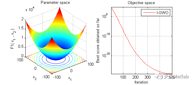
figure('Position',[500 500 660 290])
 %Draw search space
 subplot(1,2,1);
 func_plot(Function_name);
 title('Parameter space')
 xlabel('x_1');
 ylabel('x_2');
 zlabel([Function_name,'( x_1 , x_2 )'])
%Draw objective space
 subplot(1,2,2);
 semilogy(Convergence_curve,'Color','r')
 title('Objective space')
 xlabel('Iteration');
 ylabel('Best score obtained so far');
axis tight
 grid on
 box on
 legend('I-GWO')
% You can simply define your cost in a seperate file and load its handle to fobj
 % The initial parameters that you need are:
 %__________________________________________
 % fobj = @YourCostFunction
 % dim = number of your variables
 % Max_iteration = maximum number of generations
 % N = number of search agents
 % lb=[lb1,lb2,...,lbn] where lbn is the lower bound of variable n
 % ub=[ub1,ub2,...,ubn] where ubn is the upper bound of variable n
 % If all the variables have equal lower bound you can just
 % define lb and ub as two single number numbers
% To run I-GWO: [Best_score,Best_pos,GWO_cg_curve]=IGWO(SearchAgents_no,Max_iteration,lb,ub,dim,fobj)
 %__________________________________________
close all
 clear
 clc
Algorithm_Name = 'I-GWO';
N = 30; % Number of search agents
 Function_name='F2'; % Name of the test function that can be from F1 to F23 (Table 1,2,3 in the paper)
 Max_iteration = 500; % Maximum numbef of iterations
% Load details of the selected benchmark function
 [lb,ub,dim,fobj]=Get_Functions_details(Function_name);
[Fbest,Lbest,Convergence_curve]=IGWO(dim,N,Max_iteration,lb,ub,fobj);
 display(['The best solution obtained by I-GWO is : ', num2str(Lbest)]);
 display(['The best optimal value of the objective funciton found by I-GWO is : ', num2str(Fbest)]);
figure('Position',[500 500 660 290])
 %Draw search space
 subplot(1,2,1);
 func_plot(Function_name);
 title('Parameter space')
 xlabel('x_1');
 ylabel('x_2');
 zlabel([Function_name,'( x_1 , x_2 )'])
%Draw objective space
 subplot(1,2,2);
 semilogy(Convergence_curve,'Color','r')
 title('Objective space')
 xlabel('Iteration');
 ylabel('Best score obtained so far');
axis tight
 grid on
 box on
 legend('I-GWO')
3 运行结果

4 参考文献
[1]唐宏伟. 未知环境下基于智能优化算法的多机器人目标搜索研究[D]. 湖南大学.
[2]崔明朗, 杜海文, 魏政磊,等. 多目标灰狼优化算法的改进策略研究[J]. 计算机工程与应用, 2018, 54(5):9.
博主简介:擅长智能优化算法、神经网络预测、信号处理、元胞自动机、图像处理、路径规划、无人机等多种领域的Matlab仿真,相关matlab代码问题可私信交流。
部分理论引用网络文献,若有侵权联系博主删除。