Revisiting Single Image Depth Estimation Toward Higher Resolution Maps

目录

1.作者

2.论文整体结构

3.损失函数

3.1. Loss_depth

3.2. Loss_grad

3.3. Loss_normal

---

---

1.作者

2.论文整体结构

本文作者的主要贡献是针对边界扭曲，失真等问题，级联了三种损失函数共同制约网络。

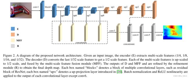
前向传播过程
1.  在Encoder 得到的四种分辨率不同的特征图，c1,c2,c3,c4.
2.  MFF模块是将c1,c2,c3,c4统一上采样到相同分辨率，然后进行concat拼接，作为MFF的输出.
3.  D模块就是将c4逐层使用双线性插值上采样到MFF输出的分辨率.
4.  D和MFF拼接之后经过多次卷积得到最终输出.

模型比较简单，基本上就是级联了多个3x3卷积和5x5卷积,毕竟是18年的文章。而这篇文章主要的创新点就是在损失函数这一块，比较有特点，引用量也达到了200+.

3.损失函数

论文使用了3种损失函数共同制约网络，分别是L1损失，grad损失，以及法线normal损失。

3.1. Loss_depth

相对于传统的 L1 损失，作者使用了 log 空间下的损失，原因是因为距离拍摄源相对远的位置，即使是相同大小的物体，在成像之后，二者占据空间大小不同。比如下面这个图中，后方的人只占据了帽子大小的像素空间。因此后方人的深度位置较难准确估计出，并且后方像素值较大，相对误差也较大。而 Log 函数抑制了这一现象，让附近点损失贡献更大，远处点损失贡献小一点。 右图坐标系x是predict与GT的差值，可以看到loss更关注拍摄源附近点。（例子可能不太适合，不是室内）

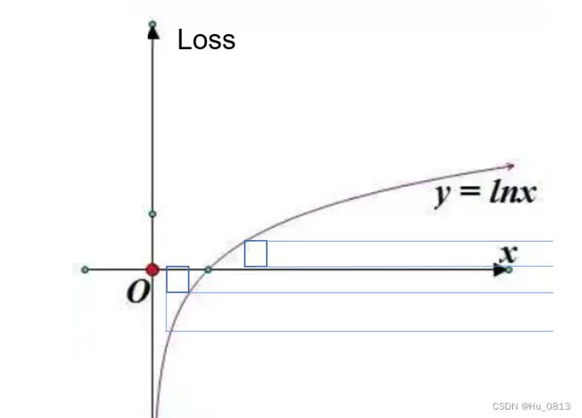
，where F = ln( || predict - Gt || + 0.05)

3.2. Loss_grad

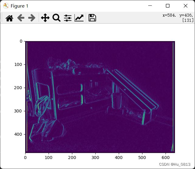
作者使用sobel算子提取预测图和GT之间的梯度做比较，进一步让网络注意到梯度信息。这一部分可以直接看代码。个人感觉在计算dx，dy的时候应该加上绝对值。左下图是不加绝对值

class Sobel(nn.Module):
    def __init__(self):
        super(Sobel, self).__init__()
        self.edge_conv = nn.Conv2d(1, 2, kernel_size=3, stride=1, padding=1, bias=False)
        edge_kx = np.array([[1, 0, -1], [2, 0, -2], [1, 0, -1]])
        edge_ky = np.array([[1, 2, 1], [0, 0, 0], [-1, -2, -1]])
        edge_k = np.stack((edge_kx, edge_ky))

        edge_k = torch.from_numpy(edge_k).float().view(2, 1, 3, 3)
        self.edge_conv.weight = nn.Parameter(edge_k)
        
        for param in self.parameters():
            param.requires_grad = False

    def forward(self, x):
        out = self.edge_conv(x)
        out = out.contiguous().view(-1, 2, x.size(2), x.size(3))
  
        return out

get_gradient = Sobel()

depth_grad = get_gradient(depth)
output_grad = get_gradient(output)
depth_grad_dx = depth_grad[:, 0, :, :].contiguous().view_as(depth)
depth_grad_dy = depth_grad[:, 1, :, :].contiguous().view_as(depth)
output_grad_dx = output_grad[:, 0, :, :].contiguous().view_as(depth)
output_grad_dy = output_grad[:, 1, :, :].contiguous().view_as(depth)

loss_dx = torch.log(torch.abs(output_grad_dx - depth_grad_dx) + 0.5).mean()
loss_dy = torch.log(torch.abs(output_grad_dy - depth_grad_dy) + 0.5).mean()
loss_grad = loss_dx + loss_dy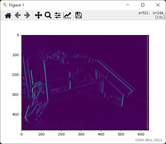

                             

3.3. Loss_normal

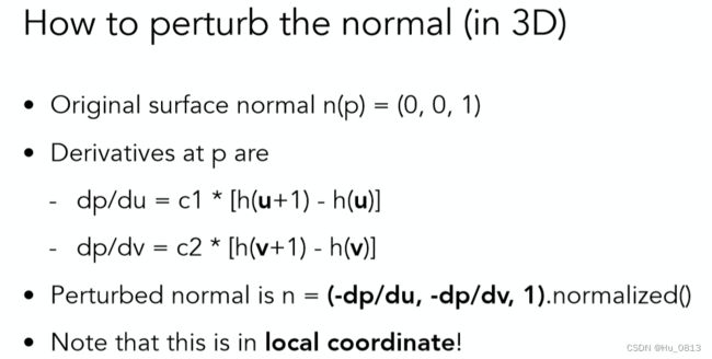
看公式不好理解，可以看代码，代码比较容易理解多了。本文normal是通过Bump Maps求解。
Bump Maps存储的是该点逻辑上的相对高度(可为负值，本文深度图的结果被归一化到了(0-1)之间，与现在流行的转化为现实距离（0-10）不同，该高度的变化实际上表现了物体表面凹凸不平的特质，利用该高度信息，再计算出该点法线向量。
直接引用计算机图形学里的内容（How to perturb the normal）
在计算出法线向量之后，作者又使用了cos函数计算了两个法线之间的角度：（1 - 余弦相似度）
余弦相似度更加注重两个向量在方向上的差异，而非距离或长度上(其实我认为也可以做减法,可以尝试一下。如下图的空间坐标系，假设predict 点A 与 GT对应点B，在方向上重合，那B可能比A的欧式距离更长，而且CNN具有平移不变性，感觉方向上没什么问题。个人猜测，可以私信我探讨。)

         

depth_normal = torch.cat((-depth_grad_dx, -depth_grad_dy, ones), 1)
output_normal = torch.cat((-output_grad_dx, -output_grad_dy, ones), 1)
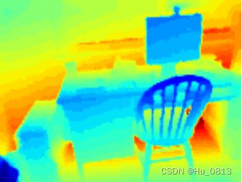
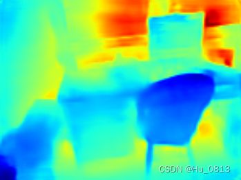
loss_normal = torch.abs(1 - cos(output_normal, depth_normal)).mean()

为了证明三种损失的有效性，消融对比如下 from left to right : GT, Predict of Ldepth, predict of Loss_all

    

 Reference

 衡量两个向量相似度的方法：余弦相似度_code_learne的博客-CSDN博客_向量余弦相似度
 闫令琪《现代计算机图形学入门》