高光谱图像分类

这次和上次情况差不多，写这篇文章的本意也是因为老师布置的作业。按要求，阅读论文《HybridSN: Exploring 3-D–2-DCNN Feature Hierarchy for Hyperspectral Image Classification》，并对里面的模型（主要是网络部分）进行复现。同时对一些问题进行思考。
当然，实验的平台仍然是谷歌的Colab（毕竟能白piao何乐而不为呢，但使用GPU时要注意使用的时间不要过长等问题，免得被限制）。语言使用的是python，网络实现所用的是pytorch。

一、准备数据

1.首先取得数据，并引入基本函数库。

! wget http://www.ehu.eus/ccwintco/uploads/6/67/Indian_pines_corrected.mat
! wget http://www.ehu.eus/ccwintco/uploads/c/c4/Indian_pines_gt.mat
! pip install spectral

如果想在自己的win上运行，也可以直接复制网址到浏览器，浏览器会自动下载的。

运行结果：

2.导入相应的函数库。

import numpy as np
import matplotlib.pyplot as plt
import scipy.io as sio
from sklearn.decomposition import PCA
from sklearn.model_selection import train_test_split
from sklearn.metrics import confusion_matrix, accuracy_score, classification_report, cohen_kappa_score
import spectral
import torch
import torchvision
import torch.nn as nn
import torch.nn.functional as F
import torch.optim as optim

二、模型的实现

1.论文中模型的定义

三维卷积部分：

conv1：（1, 30, 25, 25）， 8个 7x3x3 的卷积核 ==>（8, 24, 23, 23）
conv2：（8, 24, 23, 23）， 16个 5x3x3 的卷积核 ==>（16, 20, 21, 21）
conv3：（16, 20, 21, 21），32个 3x3x3 的卷积核 ==>（32, 18, 19, 19）
接下来要进行二维卷积，因此把前面的 32*18 reshape 一下，得到 （576, 19, 19）

二维卷积：（576, 19, 19） 64个 3x3 的卷积核，得到 （64, 17, 17）

接下来是一个 flatten 操作，变为 18496 维的向量，

接下来依次为256，128节点的全连接层，都使用比例为0.4的 Dropout，

最后输出为 16 个节点，是最终的分类类别数。

2.按定义实现 HybridSN 模型。

class_num = 16

class HybridSN(nn.Module):
  def __init__(self):
    super(HybridSN, self).__init__()
    self.conv3d_1 = nn.Sequential(
        nn.Conv3d(1, 8, kernel_size=(7, 3, 3), stride=1, padding=0),
        nn.BatchNorm3d(8),
        nn.ReLU(inplace = True),
    )
    self.conv3d_2 = nn.Sequential(
        nn.Conv3d(8, 16, kernel_size=(5, 3, 3), stride=1, padding=0),
        nn.BatchNorm3d(16),
        nn.ReLU(inplace = True),
    ) 
    self.conv3d_3 = nn.Sequential(
        nn.Conv3d(16, 32, kernel_size=(3, 3, 3), stride=1, padding=0),
        nn.BatchNorm3d(32),
        nn.ReLU(inplace = True)
    )

    self.conv2d_4 = nn.Sequential(
        nn.Conv2d(576, 64, kernel_size=(3, 3), stride=1, padding=0),
        nn.BatchNorm2d(64),
        nn.ReLU(inplace = True),
    )
    self.fc1 = nn.Linear(18496,256)
    self.fc2 = nn.Linear(256,128)
    self.fc3 = nn.Linear(128,class_num)
    self.dropout = nn.Dropout(p = 0.4)

  def forward(self,x):
    out = self.conv3d_1(x)
    out = self.conv3d_2(out)
    out = self.conv3d_3(out)
    out = self.conv2d_4(out.reshape(out.shape[0],-1,19,19))
    out = out.reshape(out.shape[0],-1)
    out = F.relu(self.dropout(self.fc1(out)))
    out = F.relu(self.dropout(self.fc2(out)))
    out = self.fc3(out)
    return out

#随机输入，测试网络结构是否通
x = torch.randn(1, 1, 30, 25, 25)
net = HybridSN()
y = net(x)
print(y.shape)

运行结果：

三、创建数据集

首先对高光谱数据实施PCA降维；然后创建 keras 方便处理的数据格式；然后随机抽取 10% 数据做为训练集，剩余的做为测试集。

1.首先定义基本函数：

# 对高光谱数据 X 应用 PCA 变换
def applyPCA(X, numComponents):
    newX = np.reshape(X, (-1, X.shape[2]))
    pca = PCA(n_components=numComponents, whiten=True)
    newX = pca.fit_transform(newX)
    newX = np.reshape(newX, (X.shape[0], X.shape[1], numComponents))
    return newX

# 对单个像素周围提取 patch 时，边缘像素就无法取了，因此，给这部分像素进行 padding 操作
def padWithZeros(X, margin=2):
    newX = np.zeros((X.shape[0] + 2 * margin, X.shape[1] + 2* margin, X.shape[2]))
    x_offset = margin
    y_offset = margin
    newX[x_offset:X.shape[0] + x_offset, y_offset:X.shape[1] + y_offset, :] = X
    return newX

# 在每个像素周围提取 patch ，然后创建成符合 keras 处理的格式
def createImageCubes(X, y, windowSize=5, removeZeroLabels = True):
    # 给 X 做 padding
    margin = int((windowSize - 1) / 2)
    zeroPaddedX = padWithZeros(X, margin=margin)
    # split patches
    patchesData = np.zeros((X.shape[0] * X.shape[1], windowSize, windowSize, X.shape[2]))
    patchesLabels = np.zeros((X.shape[0] * X.shape[1]))
    patchIndex = 0
    for r in range(margin, zeroPaddedX.shape[0] - margin):
        for c in range(margin, zeroPaddedX.shape[1] - margin):
            patch = zeroPaddedX[r - margin:r + margin + 1, c - margin:c + margin + 1]   
            patchesData[patchIndex, :, :, :] = patch
            patchesLabels[patchIndex] = y[r-margin, c-margin]
            patchIndex = patchIndex + 1
    if removeZeroLabels:
        patchesData = patchesData[patchesLabels>0,:,:,:]
        patchesLabels = patchesLabels[patchesLabels>0]
        patchesLabels -= 1
    return patchesData, patchesLabels

def splitTrainTestSet(X, y, testRatio, randomState=345):
    X_train, X_test, y_train, y_test = train_test_split(X, y, test_size=testRatio, random_state=randomState, stratify=y)
    return X_train, X_test, y_train, y_test

2.下面读取并创建数据集：

# 地物类别
class_num = 16
X = sio.loadmat('Indian_pines_corrected.mat')['indian_pines_corrected']
y = sio.loadmat('Indian_pines_gt.mat')['indian_pines_gt']

# 用于测试样本的比例
test_ratio = 0.90
# 每个像素周围提取 patch 的尺寸
patch_size = 25
# 使用 PCA 降维，得到主成分的数量
pca_components = 30

print('Hyperspectral data shape: ', X.shape)
print('Label shape: ', y.shape)

print('\n... ... PCA tranformation ... ...')
X_pca = applyPCA(X, numComponents=pca_components)
print('Data shape after PCA: ', X_pca.shape)

print('\n... ... create data cubes ... ...')
X_pca, y = createImageCubes(X_pca, y, windowSize=patch_size)
print('Data cube X shape: ', X_pca.shape)
print('Data cube y shape: ', y.shape)

print('\n... ... create train & test data ... ...')
Xtrain, Xtest, ytrain, ytest = splitTrainTestSet(X_pca, y, test_ratio)
print('Xtrain shape: ', Xtrain.shape)
print('Xtest  shape: ', Xtest.shape)

# 改变 Xtrain, Ytrain 的形状，以符合 keras 的要求
Xtrain = Xtrain.reshape(-1, patch_size, patch_size, pca_components, 1)
Xtest  = Xtest.reshape(-1, patch_size, patch_size, pca_components, 1)
print('before transpose: Xtrain shape: ', Xtrain.shape) 
print('before transpose: Xtest  shape: ', Xtest.shape) 

# 为了适应 pytorch 结构，数据要做 transpose
Xtrain = Xtrain.transpose(0, 4, 3, 1, 2)
Xtest  = Xtest.transpose(0, 4, 3, 1, 2)
print('after transpose: Xtrain shape: ', Xtrain.shape) 
print('after transpose: Xtest  shape: ', Xtest.shape) 


""" Training dataset"""
class TrainDS(torch.utils.data.Dataset): 
    def __init__(self):
        self.len = Xtrain.shape[0]
        self.x_data = torch.FloatTensor(Xtrain)
        self.y_data = torch.LongTensor(ytrain)        
    def __getitem__(self, index):
        # 根据索引返回数据和对应的标签
        return self.x_data[index], self.y_data[index]
    def __len__(self): 
        # 返回文件数据的数目
        return self.len

""" Testing dataset"""
class TestDS(torch.utils.data.Dataset): 
    def __init__(self):
        self.len = Xtest.shape[0]
        self.x_data = torch.FloatTensor(Xtest)
        self.y_data = torch.LongTensor(ytest)
    def __getitem__(self, index):
        # 根据索引返回数据和对应的标签
        return self.x_data[index], self.y_data[index]
    def __len__(self): 
        # 返回文件数据的数目
        return self.len

# 创建 trainloader 和 testloader
trainset = TrainDS()
testset  = TestDS()
train_loader = torch.utils.data.DataLoader(dataset=trainset, batch_size=128, shuffle=True, num_workers=2)
test_loader  = torch.utils.data.DataLoader(dataset=testset,  batch_size=128, shuffle=False, num_workers=2)

运行结果：

三、模型训练及测试

1.模型的训练

# 使用GPU训练，可以在菜单 "代码执行工具" -> "更改运行时类型" 里进行设置
device = torch.device("cuda:0" if torch.cuda.is_available() else "cpu")

# 网络放到GPU上
net = HybridSN().to(device)
criterion = nn.CrossEntropyLoss()
optimizer = optim.Adam(net.parameters(), lr=0.001)

# 开始训练
total_loss = 0
for epoch in range(100):
    for i, (inputs, labels) in enumerate(train_loader):
        inputs = inputs.to(device)
        labels = labels.to(device)
        # 优化器梯度归零
        optimizer.zero_grad()
        # 正向传播 +　反向传播 + 优化 
        outputs = net(inputs)
        loss = criterion(outputs, labels)
        loss.backward()
        optimizer.step()
        total_loss += loss.item()
    print('[Epoch: %d]   [loss avg: %.4f]   [current loss: %.4f]' %(epoch + 1, total_loss/(epoch+1), loss.item()))

print('Finished Training')

运行结果：

2.模型的测试

count = 0
# 模型测试
for inputs, _ in test_loader:
    inputs = inputs.to(device)
    outputs = net(inputs)
    outputs = np.argmax(outputs.detach().cpu().numpy(), axis=1)
    if count == 0:
        y_pred_test =  outputs
        count = 1
    else:
        y_pred_test = np.concatenate( (y_pred_test, outputs) )

# 生成分类报告
classification = classification_report(ytest, y_pred_test, digits=4)
print(classification)

运行结果：

五、一些备用函数

1.下面是用于计算各个类准确率，显示结果的备用函数，以供参考

from operator import truediv

def AA_andEachClassAccuracy(confusion_matrix):
    counter = confusion_matrix.shape[0]
    list_diag = np.diag(confusion_matrix)
    list_raw_sum = np.sum(confusion_matrix, axis=1)
    each_acc = np.nan_to_num(truediv(list_diag, list_raw_sum))
    average_acc = np.mean(each_acc)
    return each_acc, average_acc


def reports (test_loader, y_test, name):
    count = 0
    # 模型测试
    for inputs, _ in test_loader:
        inputs = inputs.to(device)
        outputs = net(inputs)
        outputs = np.argmax(outputs.detach().cpu().numpy(), axis=1)
        if count == 0:
            y_pred =  outputs
            count = 1
        else:
            y_pred = np.concatenate( (y_pred, outputs) )

    if name == 'IP':
        target_names = ['Alfalfa', 'Corn-notill', 'Corn-mintill', 'Corn'
                        ,'Grass-pasture', 'Grass-trees', 'Grass-pasture-mowed', 
                        'Hay-windrowed', 'Oats', 'Soybean-notill', 'Soybean-mintill',
                        'Soybean-clean', 'Wheat', 'Woods', 'Buildings-Grass-Trees-Drives',
                        'Stone-Steel-Towers']
    elif name == 'SA':
        target_names = ['Brocoli_green_weeds_1','Brocoli_green_weeds_2','Fallow','Fallow_rough_plow','Fallow_smooth',
                        'Stubble','Celery','Grapes_untrained','Soil_vinyard_develop','Corn_senesced_green_weeds',
                        'Lettuce_romaine_4wk','Lettuce_romaine_5wk','Lettuce_romaine_6wk','Lettuce_romaine_7wk',
                        'Vinyard_untrained','Vinyard_vertical_trellis']
    elif name == 'PU':
        target_names = ['Asphalt','Meadows','Gravel','Trees', 'Painted metal sheets','Bare Soil','Bitumen',
                        'Self-Blocking Bricks','Shadows']
    
    classification = classification_report(y_test, y_pred, target_names=target_names)
    oa = accuracy_score(y_test, y_pred)
    confusion = confusion_matrix(y_test, y_pred)
    each_acc, aa = AA_andEachClassAccuracy(confusion)
    kappa = cohen_kappa_score(y_test, y_pred)
    
    return classification, confusion, oa*100, each_acc*100, aa*100, kappa*100

2.检测结果写在文件里：

classification, confusion, oa, each_acc, aa, kappa = reports(test_loader, ytest, 'IP')
classification = str(classification)
confusion = str(confusion)
file_name = "classification_report.txt"

with open(file_name, 'w') as x_file:
    x_file.write('\n')
    x_file.write('{} Kappa accuracy (%)'.format(kappa))
    x_file.write('\n')
    x_file.write('{} Overall accuracy (%)'.format(oa))
    x_file.write('\n')
    x_file.write('{} Average accuracy (%)'.format(aa))
    x_file.write('\n')
    x_file.write('\n')
    x_file.write('{}'.format(classification))
    x_file.write('\n')
    x_file.write('{}'.format(confusion))

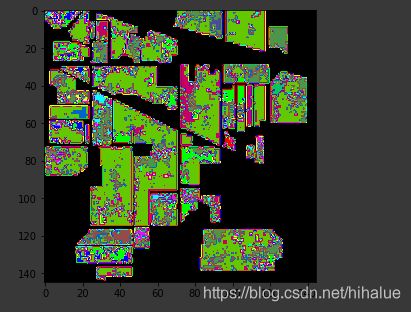
2.下面代码用于显示分类结果：

# load the original image
X = sio.loadmat('Indian_pines_corrected.mat')['indian_pines_corrected']
y = sio.loadmat('Indian_pines_gt.mat')['indian_pines_gt']

height = y.shape[0]
width = y.shape[1]

X = applyPCA(X, numComponents= pca_components)
X = padWithZeros(X, patch_size//2)

# 逐像素预测类别
outputs = np.zeros((height,width))
for i in range(height):
    for j in range(width):
        if int(y[i,j]) == 0:
            continue
        else :
            image_patch = X[i:i+patch_size, j:j+patch_size, :]
            image_patch = image_patch.reshape(1,image_patch.shape[0],image_patch.shape[1], image_patch.shape[2], 1)
            X_test_image = torch.FloatTensor(image_patch.transpose(0, 4, 3, 1, 2)).to(device)                                   
            prediction = net(X_test_image)
            prediction = np.argmax(prediction.detach().cpu().numpy(), axis=1)
            outputs[i][j] = prediction+1
    if i % 20 == 0:
        print('... ... row ', i, ' handling ... ...')

predict_image = spectral.imshow(classes = outputs.astype(int),figsize =(5,5))

运行结果：

六、对一些问题的思考

1.关于模型的预测结果不同的思考
首先，就是不同训练出来的结果不同，这很正常。
下面是另外一次训练的预测结果：

但是，同一次训练出来的模型，预测结果也会不同。
下面是和上图一样的训练模型，但结果却不同：

这里，我也查阅了一些资料。所了解到的导致这种每次测试结果会不同的原因是：
在pytorch中，网络有train和eval两种模式。
在训练模式model.train():启用BatchNormalization和Dropout；
但在测试模式model.eval():不启用BatchNormalization和Dropout。
所以，这会导致我们训练好的模型在每次测试中是不同的。

2.加入注意力机制
关于注意力机制，就不在这里详述，大家有兴趣可以去搜相关的知识进行学习。
简单来说，注意力机制可以让我们的模型更多关注图像的某一些部位，而对其他的部位不太关心。
这样可以使我们的模型关注更有价值的部分，理论上讲所得模型的精度会更好。
在这个网络模型加入注意力机制也不难，比如在二维卷积部分引入注意力机制。
下面是注意力机制的一个实现：

# 引入注意力机制
class_num = 16


class Attention_Block(nn.Module):

    def __init__(self, planes, size):
        super(Attention_Block, self).__init__()

        self.globalAvgPool = nn.AvgPool2d(size, stride=1)

        self.fc1 = nn.Linear(planes, round(planes / 16))
        self.relu = nn.ReLU()
        self.fc2 = nn.Linear(round(planes / 16), planes)
        self.sigmoid = nn.Sigmoid()

    def forward(self, x):
        residual = x

        out = self.globalAvgPool(x)
        out = out.view(out.shape[0], out.shape[1])
        out = self.fc1(out)
        out = self.relu(out)
        out = self.fc2(out)
        out = self.sigmoid(out)
        
        out = out.view(out.shape[0], out.shape[1], 1, 1)
        out = out * residual

        return out



class HybridSN(nn.Module):

    def __init__(self):
        super(HybridSN, self).__init__()
        # 3个3D卷积
        # conv1：（1, 30, 25, 25）， 8个 7x3x3 的卷积核 ==> （8, 24, 23, 23）
        self.conv3d_1 = nn.Sequential(
            nn.Conv3d(1, 8, kernel_size=(7, 3, 3), stride=1, padding=0),
            nn.BatchNorm3d(8),
            nn.ReLU(inplace = True),
            )
        # conv2：（8, 24, 23, 23）， 16个 5x3x3 的卷积核 ==>（16, 20, 21, 21）
        self.conv3d_2 = nn.Sequential(
            nn.Conv3d(8, 16, kernel_size=(5, 3, 3), stride=1, padding=0),
            nn.BatchNorm3d(16),
            nn.ReLU(inplace = True),
            ) 
        # conv3：（16, 20, 21, 21），32个 3x3x3 的卷积核 ==>（32, 18, 19, 19）
        self.conv3d_3 = nn.Sequential(
            nn.Conv3d(16, 32, kernel_size=(3, 3, 3), stride=1, padding=0),
            nn.BatchNorm3d(32),
            nn.ReLU()
            )
        # 二维卷积：（576, 19, 19） 64个 3x3 的卷积核，得到 （64, 17, 17）
        self.conv4d_2 = nn.Sequential(
            nn.Conv2d(576,64,(3,3)),
            nn.BatchNorm2d(64),
            nn.ReLU()
        )
        # 注意力机制部分
        self.layer1 = self.make_layer(Attention_Block,planes = 576, size = 19)
        self.layer2 = self.make_layer(Attention_Block,planes = 64, size = 17)

        # 接下来依次为256，128节点的全连接层，都使用比例为0.1的 Dropout
        self.fn1 = nn.Linear(18496,256)
        self.fn2 = nn.Linear(256,128)

        self.fn_out = nn.Linear(128,class_num)

        self.drop = nn.Dropout(p = 0.1)
        

    def make_layer(self, block, planes, size):
        layers = []
        layers.append(block(planes, size))
        return nn.Sequential(*layers)

    def forward(self, x):
        out = self.conv3d_1(x)
        out = self.conv3d_2(out)
        out = self.conv3d_3(out)
        # 进行二维卷积，因此把前面的 32*18 reshape 一下，得到 （576, 19, 19）
        out = out.view(out.shape[0],out.shape[1]*out.shape[2],out.shape[3],out.shape[4])

        # 在二维卷积部分引入注意力机制
        out = self.layer1(out)
        out = self.conv4d_2(out)
        out = self.layer2(out)
        # 接下来是一个 flatten 操作，变为 18496 维的向量
        # 进行重组，以b行，d列的形式存放（d自动计算）
        out = out.view(out.shape[0],-1)

        out = self.fn1(out)
        out = self.drop(out)
        out = self.fn2(out)
        out = self.drop(out)
        
        out = self.fn_out(out)

        # out = self.soft(out)

        return out

# 随机输入，测试网络结构是否通
x = torch.randn(1, 1, 30, 25, 25)
net = HybridSN()
y = net(x)
print(y.shape)
print(y)

进行测试的结果如下：

可以看到准确度还是有一定的提升的（至少在我实验的时候跑出来的模型是这个结果）。

七、心得体会

本次作业总得来说比上次更花费时间。当然不是说难度上（因为大部分代码老师还是给出来了），而是要花时间去收集一些资料，当然还有包括论文的阅读。
总的来说，感觉收获比上次要大一些。