数据挖掘与分析课程笔记
数据挖掘与分析课程笔记
- 参考教材:Data Mining and Analysis : MOHAMMED J.ZAKI, WAGNER MEIRA JR.
笔记目录
- 数据挖掘与分析课程笔记
- Chapter 1 :准备
-
- 1.1 数据矩阵
- 1.2 属性
- 1.3 代数与几何的角度
-
- 1.3.1 距离与角度
- 1.3.2 算术平均与总方差
- 1.3.3 正交投影
- 1.3.4 线性相关性与维数
- 1.4 概率观点
-
- 1.4.1 二元随机变量
- 1.4.2 多元随机变量
- 1.4.3 随机样本与统计量
- Chapter 2:数值属性
-
- 2.1 一元分析
-
- 2.1.1 集中趋势量数
- 2.2.2 离差量数
- 2.2 二元分析
- 2.3 多元分析
- Chapter 5 Kernel Method:核方法
-
- 5.1 核矩阵
-
- 5.1.1 核映射的重构
- 5.1.2 特定数据的海塞核映射
- 5.2 向量核函数
- 5.3 特征空间中基本核运算
- 5.4 复杂对象的核
-
- 5.4.1 字串的谱核
- 5.4.2 图顶点的扩散核
-
- - 幂核函数
- - 指数扩散核函数
- - 纽因曼扩散核函数
- Chapter 7:降维
-
- 7.1 背景
- 7.2 主元分析:
-
- 7.2.1 最佳直线近似
- 7.2.2 最佳2-维近似
- 7.2.3 推广
- 7.2.3 Kernel PCA:核主元分析
- Chapter 14:Hierarchical Clustering 分层聚类
-
- 14.1 预备
- 14.2 团聚分层聚类
- Chapter 15:基于密度的聚类
-
- 15.1 DBSCAN 算法
- 15.2 密度估计函数(DEF)
- 15.3 DENCLUE
- Chapter 20: Linear Discriminant Analysis
-
- 20.1 Normal LDA
- 20.2 Kernel LDA:
- Chapter 21: Support Vector Machines (SVM)
-
- 21.1 支撑向量与余量
- 21.2 SVM: 线性可分情形
Chapter 1 :准备
1.1 数据矩阵
Def.1. 数据矩阵是指一个 ( n × d ) (n\times d) (n×d) 的矩阵
D = ( X 1 X 2 ⋯ X d x 1 x 11 x 12 ⋯ x 1 d x 2 x 21 x 22 ⋯ x 2 d ⋮ ⋮ ⋮ ⋱ ⋮ x n x n 1 x n 2 ⋯ x n d ) \mathbf{D}=\left(\begin{array}{c|cccc} & X_{1} & X_{2} & \cdots & X_{d} \\ \hline \mathbf{x}_{1} & x_{11} & x_{12} & \cdots & x_{1 d} \\ \mathbf{x}_{2} & x_{21} & x_{22} & \cdots & x_{2 d} \\ \vdots & \vdots & \vdots & \ddots & \vdots \\ \mathbf{x}_{n} & x_{n 1} & x_{n 2} & \cdots & x_{n d} \end{array}\right) D=⎝⎜⎜⎜⎜⎜⎛x1x2⋮xnX1x11x21⋮xn1X2x12x22⋮xn2⋯⋯⋯⋱⋯Xdx1dx2d⋮xnd⎠⎟⎟⎟⎟⎟⎞
行:实体,列:属性
Ex. 鸢尾花数据矩阵
( 萼 片 长 萼 片 宽 花 瓣 长 花 瓣 宽 类 别 X 1 X 2 X 3 X 4 X 5 x 1 5.9 3.0 4.2 1.5 云 芝 ) \left(\begin{array}{c|ccccc} & 萼片长 & 萼片宽 & 花瓣长 & 花瓣宽 & 类别 \\ & X_{1} & X_{2} & X_{3} & X_{4} & X_{5} \\ \hline \mathbf{x}_{1} & 5.9 & 3.0 & 4.2 & 1.5 & 云芝 \\ \end{array}\right) ⎝⎛x1萼片长X15.9萼片宽X23.0花瓣长X34.2花瓣宽X41.5类别X5云芝⎠⎞
1.2 属性
Def.2.
- 数值属性 是指取实数值(或整数值)的属性。
- 若数值属性的取值范围是有限集或无限可数集,则称之为离散数值属性。若只有两种取值,则称为二元属性。
- 若数值属性的取值范围不是离散的则称为连续数值属性。
Def.3. 类别属性 是指取值为符号的属性。
1.3 代数与几何的角度
假设 D \mathbf{D} D 中所有属性均为数值的,即
x i = ( x i 1 , x i 2 , … , x i d ) T ∈ R d , i = 1 , ⋯ , n \mathbf{x}_{i}=\left(x_{i 1}, x_{i 2}, \ldots, x_{i d}\right)^{T} \in \mathbb{R}^{d},i=1,\cdots,n xi=(xi1,xi2,…,xid)T∈Rd,i=1,⋯,n
或
x j = ( x 1 j , x 2 j , … , x n j ) T ∈ R n , j = 1 , ⋯ , d \mathbf{x}_{j}=\left(x_{1 j}, x_{2j}, \ldots, x_{n j}\right)^{T} \in \mathbb{R}^{n},j=1,\cdots,d xj=(x1j,x2j,…,xnj)T∈Rn,j=1,⋯,d
☆ 默认向量为列向量。
1.3.1 距离与角度
设 a , b ∈ R d \mathbf{a}, \mathbf{b} \in \mathbb{R}^{d} a,b∈Rd ,
- 点乘: a T b = ∑ i = 1 d a i b i \mathbf{a}^{T}\mathbf{b}=\sum\limits_{i=1}^{d} a_ib_i aTb=i=1∑daibi
- 长度(欧氏范数): ∣ a ∣ = a T a = ∑ i = 1 d a i 2 \left | \mathbf{a} \right | =\sqrt{\mathbf{a}^{T}\mathbf{a} } =\sqrt{\sum\limits_{i=1}^{d} a_i^2} ∣a∣=aTa=i=1∑dai2,单位化: a ∣ a ∣ \frac{\mathbf{a}}{|\mathbf{a}|} ∣a∣a
- 距离: δ ( a , b ) = ∣ ∣ a − b ∣ ∣ = ∑ i = 1 d ( a i − b i ) 2 \delta(\mathbf{a},\mathbf{b})=||\mathbf{a}-\mathbf{b}||=\sqrt{\sum\limits_{i=1}^{d}(a_i-b_i)^2} δ(a,b)=∣∣a−b∣∣=i=1∑d(ai−bi)2
- 角度: c o s θ = ( a ∣ a ∣ ) T ( b ∣ b ∣ ) cos \theta =(\frac{\mathbf{a}}{|\mathbf{a}|})^{T}(\frac{\mathbf{b}}{|\mathbf{b}|}) cosθ=(∣a∣a)T(∣b∣b),即单位化后作点乘
- 正交: a \mathbf{a} a 与 b \mathbf{b} b 正交,若 a T b = 0 \mathbf{a}^{T}\mathbf{b}=0 aTb=0
1.3.2 算术平均与总方差
Def.3.
-
算术平均: m e a n ( D ) = μ ^ = 1 n ∑ i = 1 n x i , ∈ R d mean(\mathbf{D})=\hat{\boldsymbol{\mu}}=\frac{1}{n} \sum\limits_{i=1}^n\mathbf{x}_i,\in \mathbb{R}^{d} mean(D)=μ^=n1i=1∑nxi,∈Rd
-
总方差: v a r ( D ) = 1 n ∑ i = 1 n δ ( x i , μ ^ ) 2 var(\mathbf{D})=\frac{1}{n} \sum\limits_{i=1}^{n} \delta\left(\mathbf{x}_{i}, \hat{\boldsymbol{\mu}}\right)^{2} var(D)=n1i=1∑nδ(xi,μ^)2
自行验证: v a r ( D ) = 1 n ∑ i = 1 n ∣ ∣ x i − μ ^ ∣ ∣ 2 = 1 n ∑ i = 1 n ∣ ∣ x i ∣ ∣ 2 − ∣ ∣ μ ^ ∣ ∣ 2 var(\mathbf{D})=\frac{1}{n} \sum\limits_{i=1}^{n}||\mathbf{x}_{i}- \hat{\boldsymbol{\mu}}||^2=\frac{1}{n} \sum\limits_{i=1}^{n}||\mathbf{x}_{i}||^2-||\hat{\boldsymbol{\mu}}||^2 var(D)=n1i=1∑n∣∣xi−μ^∣∣2=n1i=1∑n∣∣xi∣∣2−∣∣μ^∣∣2
-
中心数据矩阵: c e n t e r ( D ) = ( x 1 T − μ ^ T ⋮ x n T − μ ^ T ) center(\mathbf{D})=\begin{pmatrix} \mathbf{x}_{1}^T - \hat{\boldsymbol{\mu}}^T\\ \vdots \\ \mathbf{x}_{n}^T - \hat{\boldsymbol{\mu}}^T \end{pmatrix} center(D)=⎝⎜⎛x1T−μ^T⋮xnT−μ^T⎠⎟⎞
显然 c e n t e r ( D ) center(\mathbf{D}) center(D) 的算术平均为 0 ∈ R d \mathbf{0}\in \mathbb{R}^{d} 0∈Rd
1.3.3 正交投影
Def.4. a , b ∈ R d \mathbf{a}, \mathbf{b} \in \mathbb{R}^{d} a,b∈Rd,向量 b \mathbf{b} b 沿向量 a \mathbf{a} a 方向的正交分解是指,将 b \mathbf{b} b 写成: b = p + r \mathbf{b}= \mathbf{p}+ \mathbf{r} b=p+r。其中, p \mathbf{p} p 是指 b \mathbf{b} b 在 a \mathbf{a} a 方向上的正交投影, r \mathbf{r} r 是指 a \mathbf{a} a 与 b \mathbf{b} b 之间的垂直距离。
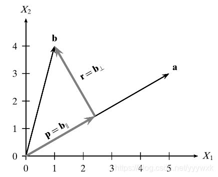
a ≠ 0 , b ≠ 0 \mathbf{a}\ne\mathbf{0},\mathbf{b}\ne\mathbf{0} a=0,b=0
设 p = c ⋅ a , ( c ≠ 0 , c ∈ R ) \mathbf{p}=c\cdot\mathbf{a},(c \ne 0,c \in \mathbb{R}) p=c⋅a,(c=0,c∈R) 则 r = b − p = b − c a \mathbf{r}=\mathbf{b}-\mathbf{p}=\mathbf{b}-c\mathbf{a} r=b−p=b−ca
0 = p T r = ( c ⋅ a ) T ( b − c a ) = c ⋅ ( a T b − c ⋅ a T a ) 0 = \mathbf{p}^T\mathbf{r} = (c\cdot\mathbf{a})^T(\mathbf{b}-c\mathbf{a})=c\cdot(\mathbf{a}^T\mathbf{b}-c\cdot\mathbf{a}^T\mathbf{a}) 0=pTr=(c⋅a)T(b−ca)=c⋅(aTb−c⋅aTa)
c = a T b a T a , p = a T b a T a ⋅ a c= \frac{\mathbf{a}^T\mathbf{b}}{\mathbf{a}^T\mathbf{a}}, \mathbf{p}=\frac{\mathbf{a}^T\mathbf{b}}{\mathbf{a}^T\mathbf{a}}\cdot\mathbf{a} c=aTaaTb,p=aTaaTb⋅a
1.3.4 线性相关性与维数
皆与线性代数相同,自读。
1.4 概率观点
每一个数值属性 X X X 被视为一个随机变量,即 X : O → R X:\mathcal{O}\rightarrow \mathbb{R} X:O→R,
其中, O \mathcal{O} O 表示 X X X 的定义域,即所有实验可能输出的集合,即样本空间。 R \mathbb{R} R : X X X 的值域,全体实数。
☆ 注:
- 随机变量是一个函数。
- 若 O \mathcal{O} O 本身是数值的(即 O ⊆ R \mathcal{O}\subseteq \mathbb{R} O⊆R,那么 X X X 是恒等函数,即 X ( v ) = v X(v)=v X(v)=v
- 若 X X X 的函数取值范围为有限集或无限可数集,则称之为离散随机变量,反之,为连续随机变量
Def.5. 若 X X X 是离散的,那么 X X X 的概率质量函数(probability mass function, PMF)为:
∀ x ∈ R , f ( x ) = P ( X = x ) \forall x \in \mathbb{R},f(x)=P(X=x) ∀x∈R,f(x)=P(X=x)
注: f ( x ) ≥ 0 , ∑ x f ( x ) = 1 f(x)\ge0,\sum\limits_xf(x)=1 f(x)≥0,x∑f(x)=1; f ( x ) = 0 f(x)=0 f(x)=0,如果 x ∉ x\notin x∈/ ( x x x 的值域)。
Def.6. 若 X X X 是连续的,那么 X X X 的概率密度函数(probability density function, PDF)为:
P ( X ∈ [ a , b ] ) = ∫ a b f ( x ) d x P(X\in [a,b])=\int_{a}^{b} f(x)dx P(X∈[a,b])=∫abf(x)dx
注: f ( x ) ≥ 0 , ∫ − ∞ + ∞ f ( x ) = 1 f(x)\ge0,\int_{-\infty}^{+\infty}f(x)=1 f(x)≥0,∫−∞+∞f(x)=1
Def.7. 对任意随机变量 X X X ,定义累积分布函数(cumulative distributution function, CDF)
F : R → [ 0 , 1 ] , ∀ x ∈ R , F ( x ) = P ( X ≤ x ) F:\mathbb{R}\to[0,1],\forall x\in \mathbb{R},F(x)=P(X\le x) F:R→[0,1],∀x∈R,F(x)=P(X≤x)
若 X X X 是离散的, F ( x ) = ∑ u ≤ x f ( u ) F(x)=\sum\limits_{u\le x}f(u) F(x)=u≤x∑f(u)
若 X X X 是连续的, F ( x ) = ∫ − ∞ x f ( u ) d u F(x)=\int_{-\infty}^xf(u)du F(x)=∫−∞xf(u)du
1.4.1 二元随机变量
X = ( X 1 X 2 ) , X : O → R 2 \mathbf{X}=\left ( \begin{matrix} X_1 \\ X_2 \end{matrix} \right ), \mathbf{X}:\mathcal{O}\to\mathbb{R}^2 X=(X1X2),X:O→R2 此处 X 1 X_1 X1, X 2 X_2 X2 分别是两个随机变量。
上课时略去了很多概念,补上。
Def.8. 若 X 1 X_1 X1 和 X 2 X_2 X2 都是离散,那么 X \mathbf{X} X 的联合概率质量函数被定义为:
f ( x ) = f ( x 1 , x 2 ) = P ( X 1 = x 1 , X 2 = x 2 ) = P ( X = x ) f(\mathbf{x})=f(x_1,x_2)=P(X_1=x_1,X_2=x_2)=P(\mathbf{X}=\mathbf{x}) f(x)=f(x1,x2)=P(X1=x1,X2=x2)=P(X=x)
注: f ( x ) ≥ 0 , ∑ x 1 ∑ x 2 f ( x 1 , x 2 ) = 1 f(x)\ge0,\sum\limits_{x_1}\sum\limits_{x_2}f(x_1,x_2)=1 f(x)≥0,x1∑x2∑f(x1,x2)=1
Def.9. 若 X 1 X_1 X1 和 X 2 X_2 X2 都是连续,那么 X \mathbf{X} X 的联合概率密度函数被定义为:
P ( X ∈ W ) = ∬ x ∈ W f ( x ) d x = ∬ ( x 1 , x 2 ) ∈ T W f ( x 1 , x 2 ) d x 1 d x 2 P(\mathbf{X} \in W)=\iint\limits_{\mathbf{x} \in W} f(\mathbf{x}) d \mathbf{x}=\iint\limits_{\left(x_{1}, x_{2}\right)^T_{\in} W} f\left(x_{1}, x_{2}\right) d x_{1} d x_{2} P(X∈W)=x∈W∬f(x)dx=(x1,x2)∈TW∬f(x1,x2)dx1dx2
其中, W ⊂ R 2 W \subset \mathbb{R}^2 W⊂R2, f ( x ) ≥ 0 , ∬ x ∈ R 2 f ( x ) d x = 1 f(\mathbf{x})\ge0,\iint\limits_{\mathbf{x}\in\mathbb{R}^2}f(\mathbf{x})d\mathbf{x}=1 f(x)≥0,x∈R2∬f(x)dx=1
Def.10. X \mathbf{X} X 的联合累积分布函数 F F F
F ( x 1 , x 2 ) = P ( X 1 ≤ x 1 and X 2 ≤ x 2 ) = P ( X ≤ x ) F(x_1,x_2)=P(X_1\le x_1 \text{ and } X_2\le x_2)=P(\mathbf{X}\le\mathbf{x}) F(x1,x2)=P(X1≤x1 and X2≤x2)=P(X≤x)
Def.11. X 1 X_1 X1 和 X 2 X_2 X2 是独立的,如果 ∀ W 1 ⊂ R \forall W_1\subset \mathbb{R} ∀W1⊂R 及 ∀ W 2 ⊂ R \forall W_2\subset \mathbb{R} ∀W2⊂R
P ( X 1 ∈ W 1 and X 2 ∈ W 2 ) = P ( X 1 ∈ W 1 ) ⋅ ( X 2 ∈ W 2 ) P(X_1\in W_1 \text{ and } X_2\in W_2)=P(X_1\in W_1)\cdot(X_2\in W_2) P(X1∈W1 and X2∈W2)=P(X1∈W1)⋅(X2∈W2)
Prop. 如果 X 1 X_1 X1 和 X 2 X_2 X2 是独立的,那么
F ( x 1 , x 2 ) = F 1 ( x 1 ) ⋅ F 2 ( x 2 ) f ( x 1 , x 2 ) = f 1 ( x 1 ) ⋅ f 2 ( x 2 ) F(x_1,x_2)=F_1(x_1)\cdot F_2(x_2)\\ f(x_1,x_2)=f_1(x_1)\cdot f_2(x_2) F(x1,x2)=F1(x1)⋅F2(x2)f(x1,x2)=f1(x1)⋅f2(x2)
其中 F i F_i Fi 是 X i X_i Xi 的累积分布函数, f i f_i fi 是 x i x_i xi 的 PMF 或 PDF。
1.4.2 多元随机变量
平行推广1.4.1节中的各定义即可。
1.4.3 随机样本与统计量
Def.12. 给定随机变量 X X X ,来源于 X X X 的长度为 n n n 的随机样本是指 n n n 个独立的且同分布(均与 X X X 具有同样的 PMF 或 PDF)的随机变量 S 1 , S 2 , ⋯ , S n S_1,S_2,\cdots,S_n S1,S2,⋯,Sn。
Def.13. 统计量 θ ^ \hat{\theta} θ^ 被定义为关于随机样本的函数 θ ^ : ( S 1 , S 2 , ⋯ , S n ) → R \hat{\theta}:(S_1,S_2,\cdots,S_n)\to \mathbb{R} θ^:(S1,S2,⋯,Sn)→R
注: θ ^ \hat{\theta} θ^ 本身也是随机变量
Chapter 2:数值属性
关注代数、几何与统计观点。
2.1 一元分析
仅关注一项属性, D = ( X x 1 x 2 ⋮ x n ) , x i ∈ R \mathbf{D}=\left(\begin{array}{c} X \\ \hline x_{1} \\ x_{2} \\ \vdots \\ x_{n} \end{array}\right),x_i\in\mathbb{R} D=⎝⎜⎜⎜⎜⎜⎛Xx1x2⋮xn⎠⎟⎟⎟⎟⎟⎞,xi∈R
统计: X X X 可视为(高维)随机变量, x i x_i xi 均是恒等随机变量, x 1 , ⋯ , x n x_1,\cdots,x_n x1,⋯,xn 也看作源于 X X X 的长度为 n n n 的随机样本。
Def.1. 经验积累分布函数
Def.2. 反积累分布函数
Def.3. 随机变量 X X X 的经验概率质量函数是指
f ^ ( x ) = 1 n ∑ i = 1 n I ( x i = x ) , ∀ x i ∈ R I ( x i = x ) = { 1 , x i = x 0 , x i ≠ x \hat{f}(x)=\frac{1}{n} \sum_{i=1}^{n} I\left(x_{i} = x\right),\forall x_i \in \mathbb{R}\\ I\left(x_{i} = x\right)=\left\{\begin{matrix} 1,x_i=x\\ 0,x_i\ne x \end{matrix}\right. f^(x)=n1i=1∑nI(xi=x),∀xi∈RI(xi=x)={1,xi=x0,xi=x
2.1.1 集中趋势量数
Def.4. 离散随机变量 X X X 的期望是指: μ : = E ( X ) = ∑ x x f ( x ) \mu:=E(X) = \sum\limits_{x} xf(x) μ:=E(X)=x∑xf(x), f ( x ) f(x) f(x) 是 X X X 的PMF
连续随机变量 X X X 的期望是指: μ : = E ( X ) = ∫ − ∞ + ∞ x f ( x ) d x \mu:=E(X) = \int\limits_{-\infin}^{+\infin} xf(x)dx μ:=E(X)=−∞∫+∞xf(x)dx, f ( x ) f(x) f(x) 是 X X X 的PDF
注: E ( a X + b Y ) = a E ( X ) + b E ( Y ) E(aX+bY)=aE(X)+bE(Y) E(aX+bY)=aE(X)+bE(Y)
Def.5. X X X 的样本平均值是指 μ ^ = 1 n ∑ i = 1 n x i \hat{\mu}=\frac{1}{n} \sum\limits_{i=1}^{n}x_i μ^=n1i=1∑nxi,注 μ ^ \hat{\mu} μ^ 是 μ \mu μ 的估计量
Def.6. 一个估计量(统计量) θ ^ \hat{\theta} θ^ 被称作统计量 θ \theta θ 的无偏估计,如果 E ( θ ^ ) = θ E(\hat{\theta})=\theta E(θ^)=θ
自证:样本平均值 μ ^ \hat{\mu} μ^ 是期望 μ \mu μ 的无偏估计量, E ( x i ) = μ for all x i E(x_i)=\mu \text{ for all } x_i E(xi)=μ for all xi
Def.7. 一个估计量是稳健的,如果它不会被样本中的极值影响。(样本平均值并不是稳健的。)
Def.8. 随机变量 X X X 的中位数
Def.9. 随机变量 X X X 的样本中位数
Def.10. 随机变量 X X X 的众数, 随机变量 X X X 的样本众数
2.2.2 离差量数
Def.11. 随机变量 X X X 的极差与样本极差
Def.12. 随机变量 X X X 的四分位距,样本的四分位距
Def.13. 随机变量 X X X 的方差是
σ 2 = var ( X ) = E [ ( X − μ ) 2 ] = { ∑ x ( x − μ ) 2 f ( x ) if X is discrete ∫ − ∞ ∞ ( x − μ ) 2 f ( x ) d x if X is continuous \sigma^{2}=\operatorname{var}(X)=E\left[(X-\mu)^{2}\right]=\left\{\begin{array}{ll} \sum_{x}(x-\mu)^{2} f(x) & \text { if } X \text { is discrete } \\ \\ \int_{-\infty}^{\infty}(x-\mu)^{2} f(x) d x & \text { if } X \text { is continuous } \end{array}\right. σ2=var(X)=E[(X−μ)2]=⎩⎨⎧∑x(x−μ)2f(x)∫−∞∞(x−μ)2f(x)dx if X is discrete if X is continuous
标准差 σ \sigma σ 是指 σ 2 \sigma^2 σ2 的正的平方根。
注:方差是关于期望的第二阶动差, r r r 阶动差是指 E [ ( x − μ ) r ] E[(x-\mu)^r] E[(x−μ)r]。
性质:
- σ 2 = E ( X 2 ) − μ 2 = E ( X 2 ) − [ E ( X ) ] 2 \sigma^2=E(X^2)-\mu^2=E(X^2)-[E(X)]^2 σ2=E(X2)−μ2=E(X2)−[E(X)]2
- v a r ( X 1 + X 2 ) = v a r ( X 1 ) + v a r ( X 2 ) var(X_1+X_2)=var(X_1)+var(X_2) var(X1+X2)=var(X1)+var(X2), X 1 , X 2 X_1,X_2 X1,X2 独立
Def.14. 样本方差是 σ ^ 2 = 1 n ∑ i = 1 n ( x i − μ ^ ) 2 \hat{\sigma}^{2}=\frac{1}{n} \sum\limits_{i=1}^{n}\left(x_{i}-\hat{\mu}\right)^{2} σ^2=n1i=1∑n(xi−μ^)2,底下非 n − 1 n-1 n−1
样本方差的几何意义:考虑中心化数据矩阵
C : = ( x 1 − μ ^ x 2 − μ ^ ⋮ x n − μ ^ ) n ⋅ σ ^ 2 = ∑ i = 1 n ( x i − μ ^ ) 2 = ∣ ∣ C ∣ ∣ 2 C:=\left(\begin{array}{c} x_{1}-\hat{\mu} \\ x_{2}-\hat{\mu} \\ \vdots \\ x_{n}-\hat{\mu} \end{array}\right)\\ n\cdot \hat{\sigma}^2=\sum\limits_{i=1}^{n}\left(x_{i}-\hat{\mu}\right)^{2}=||C||^2 C:=⎝⎜⎜⎜⎛x1−μ^x2−μ^⋮xn−μ^⎠⎟⎟⎟⎞n⋅σ^2=i=1∑n(xi−μ^)2=∣∣C∣∣2
问题: X X X 的样本平均数的期望与方差?
E ( μ ^ ) = E ( 1 n ∑ i = 1 n x i ) = 1 n ∑ i = 1 n E ( x i ) = 1 n ∑ i = 1 n μ = μ E(\hat{\mu})=E(\frac{1}{n} \sum\limits_{i=1}^{n}x_i)=\frac{1}{n} \sum\limits_{i=1}^{n} E(x_i)=\frac{1}{n}\sum\limits_{i=1}^{n}\mu=\mu\\ E(μ^)=E(n1i=1∑nxi)=n1i=1∑nE(xi)=n1i=1∑nμ=μ
方差有两种方法:第一种直接展开,第二种:运用 x 1 , ⋯ , x n x_1,\cdots,x_n x1,⋯,xn 独立同分布:
v a r ( ∑ i = 1 n x i ) ) = ∑ i = 1 n v a r ( x i ) = n ⋅ σ 2 ⟹ v a r ( μ ^ ) = σ 2 n var(\sum\limits_{i=1}^{n}x_i))=\sum\limits_{i=1}^{n}var(x_i)=n\cdot \sigma^2\Longrightarrow var(\hat{\mu})=\frac{\sigma^2}{n} var(i=1∑nxi))=i=1∑nvar(xi)=n⋅σ2⟹var(μ^)=nσ2
注:样本方差是有偏估计,因为: E ( σ 2 ) = ( n − 1 n ) σ 2 → n → + ∞ σ 2 E(\sigma^2)=(\frac{n-1}{n})\sigma^2\xrightarrow{n\to +\infin}\sigma^2 E(σ2)=(nn−1)σ2n→+∞σ2
2.2 二元分析
略
2.3 多元分析
D = ( X 1 X 2 ⋯ X d x 1 x 11 x 12 ⋯ x 1 d x 2 x 21 x 22 ⋯ x 2 d ⋮ ⋮ ⋮ ⋱ ⋮ x n x n 1 x n 2 ⋯ x n d ) \mathbf{D}=\left(\begin{array}{c|cccc} & X_{1} & X_{2} & \cdots & X_{d} \\ \hline \mathbf{x}_{1} & x_{11} & x_{12} & \cdots & x_{1 d} \\ \mathbf{x}_{2} & x_{21} & x_{22} & \cdots & x_{2 d} \\ \vdots & \vdots & \vdots & \ddots & \vdots \\ \mathbf{x}_{n} & x_{n 1} & x_{n 2} & \cdots & x_{n d} \end{array}\right) D=⎝⎜⎜⎜⎜⎜⎛x1x2⋮xnX1x11x21⋮xn1X2x12x22⋮xn2⋯⋯⋯⋱⋯Xdx1dx2d⋮xnd⎠⎟⎟⎟⎟⎟⎞
可视为: X = ( X 1 , ⋯ , X d ) T \mathbf{X}=(X_1,\cdots,X_d)^T X=(X1,⋯,Xd)T
Def.15. 对于随机变量向量 X \mathbf{X} X,其期望向量为: E [ X ] = ( E [ X 1 ] E [ X 2 ] ⋮ E [ X d ] ) E[\mathbf{X}]=\left(\begin{array}{c} E\left[X_{1}\right] \\ E\left[X_{2}\right] \\ \vdots \\ E\left[X_{d}\right] \end{array}\right) E[X]=⎝⎜⎜⎜⎛E[X1]E[X2]⋮E[Xd]⎠⎟⎟⎟⎞
样本平均值为: μ ^ = 1 n ∑ i = 1 n x i , ( = m e a n ( D ) ) ∈ R d \hat{\boldsymbol{\mu}}=\frac{1}{n} \sum\limits_{i=1}^{n} \mathbf{x}_{i},(=mean(\mathbf{D})) \in \mathbb{R}^{d} μ^=n1i=1∑nxi,(=mean(D))∈Rd
Def.16. 对于 X 1 , X 2 X_1,X_2 X1,X2,定义协方差 σ 12 = E [ ( X 1 − E ( X 1 ) ) ( X 2 − E ( X 2 ) ] = E ( X 1 X 2 ) − E ( X 1 ) E ( X 2 ) \sigma_{12}=E[(X_1-E(X_1))(X_2-E(X_2)]=E(X_1X_2)-E(X_1)E(X_2) σ12=E[(X1−E(X1))(X2−E(X2)]=E(X1X2)−E(X1)E(X2)
Remark:
- σ 12 = σ 21 \sigma_{12}=\sigma_{21} σ12=σ21
- 若两者独立,则 σ 12 = 0 \sigma_{12}=0 σ12=0
Def.17. 对于随机变量向量 X = ( X 1 , ⋯ , X d ) T \mathbf{X}=(X_1,\cdots,X_d)^T X=(X1,⋯,Xd)T,定义协方差矩阵:
Σ = E [ ( X − μ ) ( X − μ ) T ] = ( σ 1 2 σ 12 ⋯ σ 1 d σ 21 σ 2 2 ⋯ σ 2 d ⋯ ⋯ ⋯ ⋯ σ d 1 σ d 2 ⋯ σ d 2 ) d × d \boldsymbol{\Sigma}=E\left[(\mathbf{X}-\boldsymbol{\mu})(\mathbf{X}-\boldsymbol{\mu})^{T}\right]=\left(\begin{array}{cccc} \sigma_{1}^{2} & \sigma_{12} & \cdots & \sigma_{1 d} \\ \sigma_{21} & \sigma_{2}^{2} & \cdots & \sigma_{2 d} \\ \cdots & \cdots & \cdots & \cdots \\ \sigma_{d 1} & \sigma_{d 2} & \cdots & \sigma_{d}^{2} \end{array}\right)_{d\times d} Σ=E[(X−μ)(X−μ)T]=⎝⎜⎜⎛σ12σ21⋯σd1σ12σ22⋯σd2⋯⋯⋯⋯σ1dσ2d⋯σd2⎠⎟⎟⎞d×d
其为对称矩阵,定义 X \mathbf{X} X 的广义方差为 d e t ( Σ ) det(\boldsymbol{\Sigma}) det(Σ)
注:
- Σ \boldsymbol{\Sigma} Σ 是实对称矩阵且半正定,即所有特征值非负, λ 1 ≥ λ 2 ⋯ ≥ λ d ≥ 0 \lambda_1\ge \lambda_2 \cdots \ge\lambda_d \ge 0 λ1≥λ2⋯≥λd≥0
- v a r ( D ) = t r ( Σ ) = σ 1 2 + ⋯ + σ d 2 var(\mathbf{D})=tr(\Sigma)=\sigma_1^2+\cdots+\sigma_d^2 var(D)=tr(Σ)=σ12+⋯+σd2
Def.18. 对于 X = ( X 1 , ⋯ , X d ) T \mathbf{X}=(X_1,\cdots,X_d)^T X=(X1,⋯,Xd)T,定义样本协方差矩阵
Σ ^ = 1 n ( Z T Z ) = 1 n ( Z 1 T Z 1 Z 1 T Z 2 ⋯ Z 1 T Z d Z 2 T Z 1 Z 2 T Z 2 ⋯ Z 2 T Z d ⋮ ⋮ ⋱ ⋮ Z d T Z 1 Z d T Z 2 ⋯ Z d T Z d ) d × d \hat{\boldsymbol{\Sigma}}=\frac{1}{n}\left(\mathbf{Z}^{T} \mathbf{Z}\right)=\frac{1}{n}\left(\begin{array}{cccc} Z_{1}^{T} Z_{1} & Z_{1}^{T} Z_{2} & \cdots & Z_{1}^{T} Z_{d} \\ Z_{2}^{T} Z_{1} & Z_{2}^{T} Z_{2} & \cdots & Z_{2}^{T} Z_{d} \\ \vdots & \vdots & \ddots & \vdots \\ Z_{d}^{T} Z_{1} & Z_{d}^{T} Z_{2} & \cdots & Z_{d}^{T} Z_{d} \end{array}\right)_{d\times d} Σ^=n1(ZTZ)=n1⎝⎜⎜⎜⎛Z1TZ1Z2TZ1⋮ZdTZ1Z1TZ2Z2TZ2⋮ZdTZ2⋯⋯⋱⋯Z1TZdZ2TZd⋮ZdTZd⎠⎟⎟⎟⎞d×d
其中
Z = D − 1 ⋅ μ ^ T = ( x 1 T − μ ^ T x 2 T − μ ^ T ⋮ x n T − μ ^ T ) = ( − z 1 T − − z 2 T − ⋮ − z n T − ) = ( ∣ ∣ ∣ Z 1 Z 2 ⋯ Z d ∣ ∣ ∣ ) \mathbf{Z}=\mathbf{D}-\mathbf{1} \cdot \hat{\boldsymbol{\mu}}^{T}=\left(\begin{array}{c} \mathbf{x}_{1}^{T}-\hat{\boldsymbol{\mu}}^{T} \\ \mathbf{x}_{2}^{T}-\hat{\boldsymbol{\mu}}^{T} \\ \vdots \\ \mathbf{x}_{n}^{T}-\hat{\boldsymbol{\mu}}^{T} \end{array}\right)=\left(\begin{array}{ccc} -& \mathbf{z}_{1}^{T} & - \\ -& \mathbf{z}_{2}^{T} & - \\ & \vdots \\ -& \mathbf{z}_{n}^{T} & - \end{array}\right)=\left(\begin{array}{cccc} \mid & \mid & & \mid \\ Z_{1} & Z_{2} & \cdots & Z_{d} \\ \mid & \mid & & \mid \end{array}\right) Z=D−1⋅μ^T=⎝⎜⎜⎜⎛x1T−μ^Tx2T−μ^T⋮xnT−μ^T⎠⎟⎟⎟⎞=⎝⎜⎜⎜⎛−−−z1Tz2T⋮znT−−−⎠⎟⎟⎟⎞=⎝⎛∣Z1∣∣Z2∣⋯∣Zd∣⎠⎞
样本总方差是 t r ( Σ ^ ) tr(\hat{\boldsymbol{\Sigma}}) tr(Σ^),广义样本方差是 d e t ( Σ ^ ) ≥ 0 det(\hat{\boldsymbol{\Sigma}})\ge0 det(Σ^)≥0
Σ ^ = 1 n ∑ i = 1 n z i z i T \hat{\boldsymbol{\Sigma}}=\frac{1}{n}\sum\limits_{i=1}^n\mathbf{z}_{i}\mathbf{z}_{i}^T Σ^=n1i=1∑nziziT
Chapter 5 Kernel Method:核方法
Example 5.1 略, ϕ ( 核 映 射 ) : Σ ∗ ( 输 入 空 间 ) → R 4 ( 特 征 空 间 ) \phi(核映射):\Sigma^*(输入空间)\to \mathbb{R}^4(特征空间) ϕ(核映射):Σ∗(输入空间)→R4(特征空间)
Def.1. 假设核映射 ϕ : I → F \phi:\mathcal{I}\to \mathcal{F} ϕ:I→F, ϕ \phi ϕ 的核函数是指 K : I × I → R K:\mathcal{I}\times\mathcal{I}\to \mathbb{R} K:I×I→R 使得 ∀ ( x i , x j ) ∈ I × I , K ( x i , x j ) = ϕ T ( x i ) ϕ ( x j ) \forall (\mathbf{x}_i,\mathbf{x}_j)\in \mathcal{I}\times\mathcal{I},K(\mathbf{x}_i,\mathbf{x}_j)=\phi^T(\mathbf{x}_i)\phi(\mathbf{x}_j) ∀(xi,xj)∈I×I,K(xi,xj)=ϕT(xi)ϕ(xj)
Example 5.2 设 ϕ : R 2 → R 3 \phi:\mathbb{R}^2\to \mathbb{R}^3 ϕ:R2→R3 使得 ∀ a = ( a 1 , a 2 ) , ϕ ( a ) = ( a 1 2 , a 2 2 , 2 a 1 a 2 ) T \forall \mathbf{a}=(a_1,a_2),\phi(\mathbf{a})=(a_1^2,a_2^2,\sqrt2a_1a_2)^T ∀a=(a1,a2),ϕ(a)=(a12,a22,2a1a2)T
注意到 K ( a , b ) = ϕ ( a ) T ϕ ( b ) = a 1 2 b 1 2 + a 2 2 b 2 2 + 2 a 1 2 a 2 2 b 1 2 b 2 2 K(\mathbf{a},\mathbf{b})=\phi(\mathbf{a})^T\phi(\mathbf{b})=a_1^2b_1^2+a_2^2b_2^2+2a_1^2a_2^2b_1^2b_2^2 K(a,b)=ϕ(a)Tϕ(b)=a12b12+a22b22+2a12a22b12b22, K : R 2 × R 2 → R K:\mathbb{R}^2\times\mathbb{R}^2\to \mathbb{R} K:R2×R2→R
Remark:
- 分析复杂数据
- 分析非线性特征(知乎搜核函数有什么作用)
Goal:在未知 ϕ \phi ϕ 的情况下,通过分析 K K K 来分析特征空间 F \mathcal{F} F 结果。
5.1 核矩阵
设 D = { x 1 , x 2 , … , x n } ⊂ I \mathbf{D}=\left\{\mathbf{x}_{1}, \mathbf{x}_{2}, \ldots, \mathbf{x}_{n}\right\} \subset \mathcal{I} D={x1,x2,…,xn}⊂I,其核矩阵定义为: K = [ K ( x i , x j ) ] n × n \mathbf{K}=[K(\mathbf{x}_{i},\mathbf{x}_{j})]_{n\times n} K=[K(xi,xj)]n×n
Prop. 核矩阵 K \mathbf{K} K 是对称的且半正定的
Proof. K ( x i , x j ) = ϕ T ( x i ) ϕ ( x j ) = ϕ T ( x j ) ϕ ( x i ) = K ( x j , x i ) K(\mathbf{x}_{i},\mathbf{x}_{j})=\phi^T(\mathbf{x}_i)\phi(\mathbf{x}_j)=\phi^T(\mathbf{x}_j)\phi(\mathbf{x}_i)=K(\mathbf{x}_{j},\mathbf{x}_{i}) K(xi,xj)=ϕT(xi)ϕ(xj)=ϕT(xj)ϕ(xi)=K(xj,xi),故对称。
对于 ∀ a T ∈ R n \forall \mathbf{a}^{T}\in \mathbb{R}^n ∀aT∈Rn,
a T K a = ∑ i = 1 n ∑ j = 1 n a i a j K ( x i , x j ) = ∑ i = 1 n ∑ j = 1 n a i a j ϕ ( x i ) T ϕ ( x j ) = ( ∑ i = 1 n a i ϕ ( x i ) ) T ( ∑ j = 1 n a j ϕ ( x j ) ) = ∥ ∑ i = 1 n a i ϕ ( x i ) ∥ 2 ≥ 0 \begin{aligned} \mathbf{a}^{T} \mathbf{K a} &=\sum_{i=1}^{n} \sum_{j=1}^{n} a_{i} a_{j} K\left(\mathbf{x}_{i}, \mathbf{x}_{j}\right) \\ &=\sum_{i=1}^{n} \sum_{j=1}^{n} a_{i} a_{j} \phi\left(\mathbf{x}_{i}\right)^{T} \phi\left(\mathbf{x}_{j}\right) \\ &=\left(\sum_{i=1}^{n} a_{i} \phi\left(\mathbf{x}_{i}\right)\right)^{T}\left(\sum_{j=1}^{n} a_{j} \phi\left(\mathbf{x}_{j}\right)\right) \\ &=\left\|\sum_{i=1}^{n} a_{i} \phi\left(\mathbf{x}_{i}\right)\right\|^2 \geq 0 \end{aligned} aTKa=i=1∑nj=1∑naiajK(xi,xj)=i=1∑nj=1∑naiajϕ(xi)Tϕ(xj)=(i=1∑naiϕ(xi))T(j=1∑najϕ(xj))=∥∥∥∥∥i=1∑naiϕ(xi)∥∥∥∥∥2≥0
5.1.1 核映射的重构
”经验核映射“
已知 D = { x i } i = 1 n ⊂ I \mathbf{D}=\left\{\mathbf{x}_{i}\right\}_{i=1}^{n} \subset \mathcal{I} D={xi}i=1n⊂I 与核矩阵 K \mathbf{K} K
目标:寻找 ϕ : I → F ⊂ R n \phi:\mathcal{I} \to \mathcal{F} \subset \mathbb{R}^n ϕ:I→F⊂Rn
首先尝试: ∀ x ∈ I , ϕ ( x ) = ( K ( x 1 , x ) , K ( x 2 , x ) , … , K ( x n , x ) ) T ∈ R n \forall \mathbf{x} \in \mathcal{I},\phi(\mathbf{x})=\left(K\left(\mathbf{x}_{1}, \mathbf{x}\right), K\left(\mathbf{x}_{2}, \mathbf{x}\right), \ldots, K\left(\mathbf{x}_{n}, \mathbf{x}\right)\right)^{T} \in \mathbb{R}^{n} ∀x∈I,ϕ(x)=(K(x1,x),K(x2,x),…,K(xn,x))T∈Rn
检查: ϕ T ( x i ) ϕ ( x j ) ? = K ( x i , x j ) \phi^T(\mathbf{x}_i)\phi(\mathbf{x}_j)?=K(\mathbf{x}_{i},\mathbf{x}_{j}) ϕT(xi)ϕ(xj)?=K(xi,xj)
左边 = ϕ ( x i ) T ϕ ( x j ) = ∑ k = 1 n K ( x k , x i ) K ( x k , x j ) = K i T K j =\phi\left(\mathbf{x}_{i}\right)^{T} \phi\left(\mathbf{x}_{j}\right)=\sum\limits_{k=1}^{n} K\left(\mathbf{x}_{k}, \mathbf{x}_{i}\right) K\left(\mathbf{x}_{k}, \mathbf{x}_{j}\right)=\mathbf{K}_{i}^{T} \mathbf{K}_{j} =ϕ(xi)Tϕ(xj)=k=1∑nK(xk,xi)K(xk,xj)=KiTKj, K i \mathbf{K}_{i} Ki 代表第 i i i 行或列要求太高。
考虑改进:寻找矩阵 A \mathbf{A} A 使得, K i T A K j = K ( x i , x j ) \mathbf{K}_{i}^{T} \mathbf{A} \mathbf{K}_{j}=\mathbf{K}\left(\mathbf{x}_{i}, \mathbf{x}_{j}\right) KiTAKj=K(xi,xj),即 K T A K = K \mathbf{K}^{T} \mathbf{A} \mathbf{K}=\mathbf{K} KTAK=K
故只需取 A = K − 1 \mathbf{A}=\mathbf{K}^{-1} A=K−1 即可( K \mathbf{K} K 可逆)
若 K \mathbf{K} K 正定, K − 1 \mathbf{K}^{-1} K−1 也正定,即存在一个实矩阵 B \mathbf{B} B 满足 K − 1 = B T B \mathbf{K}^{-1}=\mathbf{B}^{T}\mathbf{B} K−1=BTB
故经验核函数可定义为:
ϕ ( x ) = B ⋅ ( K ( x 1 , x ) , K ( x 2 , x ) , … , K ( x n , x ) ) T \phi(\mathbf{x})=\mathbf{B}\cdot\left(K\left(\mathbf{x}_{1}, \mathbf{x}\right), K\left(\mathbf{x}_{2}, \mathbf{x}\right), \ldots, K\left(\mathbf{x}_{n}, \mathbf{x}\right)\right)^{T} ϕ(x)=B⋅(K(x1,x),K(x2,x),…,K(xn,x))T
检查: ϕ T ( x i ) ϕ ( x j ) = ( B K i ) T ( B K j ) = K i T K − 1 K j = ( K T K − 1 K ) i , j = K ( x i , x j ) \phi^T(\mathbf{x}_i)\phi(\mathbf{x}_j)=(\mathbf{B}\mathbf{K}_i)^T(\mathbf{B}\mathbf{K}_j)=\mathbf{K}_i^T\mathbf{K}^{-1}\mathbf{K}_j=(\mathbf{K}^T\mathbf{K}^{-1}\mathbf{K})_{i,j}=K(\mathbf{x}_{i},\mathbf{x}_{j}) ϕT(xi)ϕ(xj)=(BKi)T(BKj)=KiTK−1Kj=(KTK−1K)i,j=K(xi,xj)
5.1.2 特定数据的海塞核映射
对于对称半正定矩阵 K n × n \mathbf{K}_{n\times n} Kn×n,存在分解
K = U ( λ 1 0 ⋯ 0 0 λ 2 ⋯ 0 ⋮ ⋮ ⋱ ⋮ 0 0 ⋯ λ n ) U T = U Λ U T \mathbf{K}=\mathbf{U}\left(\begin{array}{cccc} \lambda_{1} & 0 & \cdots & 0 \\ 0 & \lambda_{2} & \cdots & 0 \\ \vdots & \vdots & \ddots & \vdots \\ 0 & 0 & \cdots & \lambda_{n} \end{array}\right)\mathbf{U}^{T}=\mathbf{U}\boldsymbol{\Lambda}\mathbf{U}^{T} K=U⎝⎜⎜⎜⎛λ10⋮00λ2⋮0⋯⋯⋱⋯00⋮λn⎠⎟⎟⎟⎞UT=UΛUT
λ i \lambda_{i} λi 为特征值, U = ( ∣ ∣ ∣ u 1 u 2 ⋯ u n ∣ ∣ ∣ ) \mathbf{U}=\left(\begin{array}{cccc} \mid & \mid & & \mid \\ \mathbf{u}_{1} & \mathbf{u}_{2} & \cdots & \mathbf{u}_{n} \\ \mid & \mid & & \mid \end{array}\right) U=⎝⎛∣u1∣∣u2∣⋯∣un∣⎠⎞ 为单位正交矩阵, u i = ( u i 1 , u i 2 , … , u i n ) T ∈ R n \mathbf{u}_{i}=\left(u_{i 1}, u_{i 2}, \ldots, u_{i n}\right)^{T} \in \mathbb{R}^{n} ui=(ui1,ui2,…,uin)T∈Rn 为特征向量,即
K = λ 1 u 1 u 1 T + λ 2 u 2 u 2 T + ⋯ + λ n u n u n T K ( x i , x j ) = λ 1 u 1 i u 1 j + λ 2 u 2 i u 2 j ⋯ + λ n u n i u n j = ∑ k = 1 n λ k u k i u k j \mathbf{K}=\lambda_{1} \mathbf{u}_{1} \mathbf{u}_{1}^{T}+\lambda_{2} \mathbf{u}_{2} \mathbf{u}_{2}^{T}+\cdots+\lambda_{n} \mathbf{u}_{n} \mathbf{u}_{n}^{T}\\ \begin{aligned} \mathbf{K}\left(\mathbf{x}_{i}, \mathbf{x}_{j}\right) &=\lambda_{1} u_{1 i} u_{1 j}+\lambda_{2} u_{2 i} u_{2 j} \cdots+\lambda_{n} u_{n i} u_{n j} \\ &=\sum_{k=1}^{n} \lambda_{k} u_{k i} u_{k j} \end{aligned} K=λ1u1u1T+λ2u2u2T+⋯+λnununTK(xi,xj)=λ1u1iu1j+λ2u2iu2j⋯+λnuniunj=k=1∑nλkukiukj
定义海塞映射:
∀ x i ∈ D , ϕ ( x i ) = ( λ 1 u 1 i , λ 2 u 2 i , … , λ n u n i ) T \forall \mathbf{x}_i \in \mathbf {D}, \phi\left(\mathbf{x}_{i}\right)=\left(\sqrt{\lambda_{1}} u_{1 i}, \sqrt{\lambda_{2}} u_{2 i}, \ldots, \sqrt{\lambda_{n}} u_{n i}\right)^{T} ∀xi∈D,ϕ(xi)=(λ1u1i,λ2u2i,…,λnuni)T
检查:
ϕ ( x i ) T ϕ ( x j ) = ( λ 1 u 1 i , … , λ n u n i ) ( λ 1 u 1 j , … , λ n u n j ) T = λ 1 u 1 i u 1 j + ⋯ + λ n u n i u n j = K ( x i , x j ) \begin{aligned} \phi\left(\mathbf{x}_{i}\right)^{T} \phi\left(\mathbf{x}_{j}\right) &=\left(\sqrt{\lambda_{1}} u_{1 i}, \ldots, \sqrt{\lambda_{n}} u_{n i}\right)\left(\sqrt{\lambda_{1}} u_{1 j}, \ldots, \sqrt{\lambda_{n}} u_{n j}\right)^{T} \\ &=\lambda_{1} u_{1 i} u_{1 j}+\cdots+\lambda_{n} u_{n i} u_{n j}=K\left(\mathbf{x}_{i}, \mathbf{x}_{j}\right) \end{aligned} ϕ(xi)Tϕ(xj)=(λ1u1i,…,λnuni)(λ1u1j,…,λnunj)T=λ1u1iu1j+⋯+λnuniunj=K(xi,xj)
注意:海塞映射中仅对 D \mathbf{D} D 中的数 x i \mathbf{x}_i xi 有定义。
5.2 向量核函数
R d × R d → R \mathbb{R}^d \times \mathbb{R}^d \to \mathbb{R} Rd×Rd→R
典型向量核函数:多项式核
∀ x , y ∈ R d , K q ( x , y ) = ϕ ( x ) T ϕ ( y ) = ( x T y + c ) q \forall \mathbf{x},\mathbf{y} \in \mathbb {R}^d, K_{q}(\mathbf{x}, \mathbf{y})=\phi(\mathbf{x})^{T} \phi(\mathbf{y})=\left(\mathbf{x}^{T} \mathbf{y} + c \right)^{q} ∀x,y∈Rd,Kq(x,y)=ϕ(x)Tϕ(y)=(xTy+c)q,其中 c ≥ 0 c\ge 0 c≥0
若 c = 0 c=0 c=0,齐次,否则为非齐次。
问题:构造核映射 ϕ : R d → F \phi:\mathbb{R}^d \to \mathcal{F} ϕ:Rd→F,使得 K q ( x , y ) = ϕ ( x ) T ϕ ( y ) K_{q}(\mathbf{x}, \mathbf{y})=\phi(\mathbf{x})^{T} \phi(\mathbf{y}) Kq(x,y)=ϕ(x)Tϕ(y)
注: q = 1 , c = 0 , ϕ ( x ) = x q=1,c=0, \phi (\mathbf{x})=\mathbf{x} q=1,c=0,ϕ(x)=x
示例: q = 2 , d = 2 q=2,d=2 q=2,d=2
高斯核自读
5.3 特征空间中基本核运算
ϕ : I → F , K : I × I → R \phi:\mathcal{I} \to \mathcal{F}, K:\mathcal{I} \times \mathcal{I}\to \mathbb{R} ϕ:I→F,K:I×I→R
-
向量长度: ∥ ϕ ( x ) ∥ 2 = ϕ ( x ) T ϕ ( x ) = K ( x , x ) \|\phi(\mathbf{x})\|^{2}=\phi(\mathbf{x})^{T} \phi(\mathbf{x})=K(\mathbf{x}, \mathbf{x}) ∥ϕ(x)∥2=ϕ(x)Tϕ(x)=K(x,x)
-
距离:
∥ ϕ ( x i ) − ϕ ( x j ) ∥ 2 = ∥ ϕ ( x i ) ∥ 2 + ∥ ϕ ( x j ) ∥ 2 − 2 ϕ ( x i ) T ϕ ( x j ) = K ( x i , x i ) + K ( x j , x j ) − 2 K ( x i , x j ) \begin{aligned} \left\|\phi\left(\mathbf{x}_{i}\right)-\phi\left(\mathbf{x}_{j}\right)\right\|^{2} &=\left\|\phi\left(\mathbf{x}_{i}\right)\right\|^{2}+\left\|\phi\left(\mathbf{x}_{j}\right)\right\|^{2}-2 \phi\left(\mathbf{x}_{i}\right)^{T} \phi\left(\mathbf{x}_{j}\right) \\ &=K\left(\mathbf{x}_{i}, \mathbf{x}_{i}\right)+K\left(\mathbf{x}_{j}, \mathbf{x}_{j}\right)-2 K\left(\mathbf{x}_{i}, \mathbf{x}_{j}\right) \end{aligned} ∥ϕ(xi)−ϕ(xj)∥2=∥ϕ(xi)∥2+∥ϕ(xj)∥2−2ϕ(xi)Tϕ(xj)=K(xi,xi)+K(xj,xj)−2K(xi,xj)
2 K ( x , y ) = ∥ ϕ ( x ) ∥ 2 + ∥ ϕ ( y ) ∥ 2 − ∥ ϕ ( x ) − ϕ ( y ) ∥ 2 2 K\left(\mathbf{x}, \mathbf{y}\right)=\left\|\phi\left(\mathbf{x}\right)\right\|^{2}+\left\|\phi\left(\mathbf{y}\right)\right\|^{2}-\left\|\phi\left(\mathbf{x}\right)-\phi\left(\mathbf{y}\right)\right\|^{2} 2K(x,y)=∥ϕ(x)∥2+∥ϕ(y)∥2−∥ϕ(x)−ϕ(y)∥2
代表 ϕ ( x ) \phi\left(\mathbf{x}\right) ϕ(x) 与 ϕ ( y ) \phi\left(\mathbf{y}\right) ϕ(y) 的相似度
-
平均值: μ ϕ = 1 n ∑ i = 1 n ϕ ( x i ) \boldsymbol{\mu}_{\phi}=\frac{1}{n} \sum\limits_{i=1}^{n} \phi\left(\mathbf{x}_{i}\right) μϕ=n1i=1∑nϕ(xi)
∥ μ ϕ ∥ 2 = μ ϕ T μ ϕ = ( 1 n ∑ i = 1 n ϕ ( x i ) ) T ( 1 n ∑ j = 1 n ϕ ( x j ) ) = 1 n 2 ∑ i = 1 n ∑ j = 1 n ϕ ( x i ) T ϕ ( x j ) = 1 n 2 ∑ i = 1 n ∑ j = 1 n K ( x i , x j ) \begin{aligned} \left\|\boldsymbol{\mu}_{\phi}\right\|^{2} &=\boldsymbol{\mu}_{\phi}^{T} \boldsymbol{\mu}_{\phi} \\ &=\left(\frac{1}{n} \sum\limits_{i=1}^{n} \phi\left(\mathbf{x}_{i}\right)\right)^{T}\left(\frac{1}{n} \sum\limits_{j=1}^{n} \phi\left(\mathbf{x}_{j}\right)\right) \\ &=\frac{1}{n^{2}} \sum\limits_{i=1}^{n} \sum\limits_{j=1}^{n} \phi\left(\mathbf{x}_{i}\right)^{T} \phi\left(\mathbf{x}_{j}\right) \\ &=\frac{1}{n^{2}} \sum\limits_{i=1}^{n} \sum\limits_{j=1}^{n} K\left(\mathbf{x}_{i}, \mathbf{x}_{j}\right) \end{aligned} ∥∥μϕ∥∥2=μϕTμϕ=(n1i=1∑nϕ(xi))T(n1j=1∑nϕ(xj))=n21i=1∑nj=1∑nϕ(xi)Tϕ(xj)=n21i=1∑nj=1∑nK(xi,xj) -
总方差: σ ϕ 2 = 1 n ∑ i = 1 n ∥ ϕ ( x i ) − μ ϕ ∥ 2 \sigma_{\phi}^{2}=\frac{1}{n} \sum\limits_{i=1}^{n}\left\|\phi\left(\mathbf{x}_{i}\right)-\boldsymbol{\mu}_{\phi}\right\|^{2} σϕ2=n1i=1∑n∥∥ϕ(xi)−μϕ∥∥2, ∀ x i \forall \mathbf{x}_{i} ∀xi
∥ ϕ ( x i ) − μ ϕ ∥ 2 = ∥ ϕ ( x i ) ∥ 2 − 2 ϕ ( x i ) T μ ϕ + ∥ μ ϕ ∥ 2 = K ( x i , x i ) − 2 n ∑ j = 1 n K ( x i , x j ) + 1 n 2 ∑ s = 1 n ∑ t = 1 n K ( x s , x t ) \begin{aligned} \left\|\phi\left(\mathbf{x}_{i}\right)-\boldsymbol{\mu}_{\phi}\right\|^{2} &=\left\|\phi\left(\mathbf{x}_{i}\right)\right\|^{2}-2 \phi\left(\mathbf{x}_{i}\right)^{T} \boldsymbol{\mu}_{\phi}+\left\|\boldsymbol{\mu}_{\phi}\right\|^{2} \\ &=K\left(\mathbf{x}_{i}, \mathbf{x}_{i}\right)-\frac{2}{n} \sum_{j=1}^{n} K\left(\mathbf{x}_{i}, \mathbf{x}_{j}\right)+\frac{1}{n^{2}} \sum_{s=1}^{n} \sum_{t=1}^{n} K\left(\mathbf{x}_{s}, \mathbf{x}_{t}\right) \end{aligned} ∥∥ϕ(xi)−μϕ∥∥2=∥ϕ(xi)∥2−2ϕ(xi)Tμϕ+∥∥μϕ∥∥2=K(xi,xi)−n2j=1∑nK(xi,xj)+n21s=1∑nt=1∑nK(xs,xt)σ ϕ 2 = 1 n ∑ i = 1 n ∥ ϕ ( x i ) − μ ϕ ∥ 2 = 1 n ∑ i = 1 n ( K ( x i , x i ) − 2 n ∑ j = 1 n K ( x i , x j ) + 1 n 2 ∑ s = 1 n ∑ t = 1 n K ( x s , x t ) ) = 1 n ∑ i = 1 n K ( x i , x i ) − 2 n 2 ∑ i = 1 n ∑ j = 1 n K ( x i , x j ) + 1 n 2 ∑ s = 1 n ∑ t = 1 n K ( x s , x t ) = 1 n ∑ i = 1 n K ( x i , x i ) − 1 n 2 ∑ i = 1 n ∑ j = 1 n K ( x i , x j ) \begin{aligned} \sigma_{\phi}^{2} &=\frac{1}{n} \sum\limits_{i=1}^{n}\left\|\phi\left(\mathbf{x}_{i}\right)-\boldsymbol{\mu}_{\phi}\right\|^{2}\\ &=\frac{1}{n} \sum\limits_{i=1}^{n}\left(K\left(\mathbf{x}_{i}, \mathbf{x}_{i}\right)-\frac{2}{n} \sum\limits_{j=1}^{n} K\left(\mathbf{x}_{i}, \mathbf{x}_{j}\right)+\frac{1}{n^{2}} \sum\limits_{s=1}^{n} \sum\limits_{t=1}^{n} K\left(\mathbf{x}_{s}, \mathbf{x}_{t}\right)\right)\\ &=\frac{1}{n} \sum\limits_{i=1}^{n} K\left(\mathbf{x}_{i}, \mathbf{x}_{i}\right)-\frac{2}{n^{2}} \sum\limits_{i=1}^{n} \sum\limits_{j=1}^{n} K\left(\mathbf{x}_{i}, \mathbf{x}_{j}\right)+\frac{1}{n^{2}} \sum\limits_{s=1}^{n} \sum\limits_{t=1}^{n} K\left(\mathbf{x}_{s}, \mathbf{x}_{t}\right)\\ &=\frac{1}{n} \sum\limits_{i=1}^{n} K\left(\mathbf{x}_{i}, \mathbf{x}_{i}\right)-\frac{1}{n^{2}} \sum\limits_{i=1}^{n} \sum\limits_{j=1}^{n} K\left(\mathbf{x}_{i}, \mathbf{x}_{j}\right) \end{aligned} σϕ2=n1i=1∑n∥∥ϕ(xi)−μϕ∥∥2=n1i=1∑n(K(xi,xi)−n2