【吴恩达深度学习编程作业】4.2深度卷积网络——Keras入门与残差网络的搭建

参考文章：Keras入门与残差网络的搭建
结果就是笑脸检测并不准确，手势识别也不准确。

1.Keras入门——笑脸识别

main.py

import numpy as np
import matplotlib.pyplot as plt
from matplotlib.pyplot import imshow
from keras.layers import Input, Dense, Activation, ZeroPadding2D, BatchNormalization, Flatten, Conv2D
from keras.layers import MaxPooling2D
from keras.models import Model
from keras.preprocessing import image
from keras.applications.imagenet_utils import preprocess_input
from IPython.display import SVG
from keras.utils.vis_utils import model_to_dot
from keras.utils import plot_model
import Deep_Learning.test4_2.kt_utils
import keras.backend as K
K.set_image_data_format('channels_last')


# 加载数据集
X_train_orig, Y_train_orig, X_test_orig, Y_test_orig, classes = Deep_Learning.test4_2.kt_utils.load_dataset()

# Normalize image vectors
X_train = X_train_orig / 255.
X_test = X_test_orig / 255.

# Reshape
Y_train = Y_train_orig.T
Y_test = Y_test_orig.T

print("number of training example = " + str(X_train.shape[0]))  # number of training example = 600
print("number of test example = " + str(X_test.shape[0]))       # number of test example = 150
print("X_train shape: " + str(X_train.shape))                   # X_train shape: (600, 64, 64, 3)
print("Y_train shape: " + str(Y_train.shape))                   # Y_train shape: (600, 1)
print("X_test shape: " + str(X_test.shape))                     # X_test shape: (150, 64, 64, 3)
print("Y_test shape: " + str(Y_test.shape))                     # Y_test shape: (150, 1)


"""
    Keras框架使用的变量名和以前使用的numpy和TensorFlow变量不一样。
    它不是在前向传播的每一步上创建新变量（如X, Z1, A1, Z2, A2,…）以便于不同层之间的计算。
    在Keras中使用X覆盖了所有的值，没有保存每一层结果，只需要最新的值。
    唯一例外的是X_input，将它分离出来是因为它是输入的数据，要在最后的创建模型那一步中用到。
"""

def HappyModel(input_shape):
    """
    实现一个检测笑容的模型
    :param input_shape:     -输入的数据的维度
    :return: model          -创建的Keras的模型
    """
    # 定义一个tensor的placeholder，维度为input_shape
    X_input = Input(input_shape)

    # 使用0填充X_input
    X = ZeroPadding2D((3, 3))(X_input)

    # 对X使用CONV -> BN -> RELU 块
    X = Conv2D(32, (7, 7), strides=(1, 1), name='conv0')(X)
    X = BatchNormalization(axis=3, name='bn0')(X)
    X = Activation('relu')(X)

    # 最大值池化层
    X = MaxPooling2D((2, 2), name='max_pool')(X)

    # 降维，矩阵转化为向量+全连接层
    X = Flatten()(X)
    X = Dense(1, activation='sigmoid', name='fc')(X)

    # 创建模型，可以用它来训练、测试
    model = Model(inputs=X_input, outputs=X, name='HappyModel')

    return model

"""
    训练并测试模型
"""
# 创建一个模型实体
happy_model = HappyModel(X_train.shape[1:])     # X_train.shape[1:] = (64, 64, 3)
# 编译模型：compile(self, optimizer, loss, metrics=None, loss_weights=None, sample_weight_mode=None...)
happy_model.compile("adam", "binary_crossentropy", metrics=['accuracy'])
# 训练模型：需要花费的时间很长6-10min：verbose：含义同fit的同名参数，但只能取0或1
happy_model.fit(X_train, Y_train, epochs=40, batch_size=50)
# 评估模型
preds = happy_model.evaluate(X_test, Y_test, batch_size=32, verbose=1, sample_weight=None)
print("误差值 = " + str(preds[0]))
print("准确度 = " + str(preds[1]))


"""
    如果模型准确度小于75%，可以改变模型：
        X = Conv2D(32, (3, 3), strides=(1, 1), name='conv0')(X)
        X = BatchNormalization(axis=3, name='bn0')(X)
        X = Activation('relu')(X)
       
        1.可以在每个块后面使用最大值池化层，减少宽、高的维度
        2.改变优化器，这里使用的是Adam
        3.如果模型难以运行，并且遇到了内存不够的问题，降低batch-size(12比较折中)
        4.运行更多代，直到结果满意
"""

# 测试自己的图片
img_path = 'images/smile.png'
img = image.load_img(img_path, target_size=(64, 64))
imshow(img)
plt.show()
x = image.img_to_array(img)
x = np.expand_dims(x, axis=0)
x = preprocess_input(x)
print(happy_model.predict(x))

img_path = 'images/no_smile.jpg'
img = image.load_img(img_path, target_size=(64, 64))
imshow(img)
plt.show()
x = image.img_to_array(img)
x = np.expand_dims(x, axis=0)
x = preprocess_input(x)
print(happy_model.predict(x))


# 打印每一层的大小细节
happy_model.summary()

# 绘制出布局图
plot_model(happy_model, to_file='happy_model.png')
SVG(model_to_dot(happy_model).create(prog='dot', format='svg'))

运行结果

Epoch 1/40
12/12 [==============================] - 4s 324ms/step - loss: 3.3070 - accuracy: 0.5133
Epoch 2/40
12/12 [==============================] - 4s 309ms/step - loss: 0.7813 - accuracy: 0.7283
Epoch 3/40
12/12 [==============================] - 4s 336ms/step - loss: 0.3564 - accuracy: 0.8483
Epoch 4/40
12/12 [==============================] - 3s 282ms/step - loss: 0.2107 - accuracy: 0.9217
Epoch 5/40
12/12 [==============================] - 3s 275ms/step - loss: 0.1492 - accuracy: 0.9450
Epoch 6/40
12/12 [==============================] - 4s 313ms/step - loss: 0.1323 - accuracy: 0.9550
Epoch 7/40
12/12 [==============================] - 4s 294ms/step - loss: 0.1413 - accuracy: 0.9500
Epoch 8/40
12/12 [==============================] - 3s 260ms/step - loss: 0.1208 - accuracy: 0.9550
Epoch 9/40
12/12 [==============================] - 4s 297ms/step - loss: 0.0947 - accuracy: 0.9733
Epoch 10/40
12/12 [==============================] - 3s 282ms/step - loss: 0.0863 - accuracy: 0.9783
Epoch 11/40
12/12 [==============================] - 3s 275ms/step - loss: 0.0780 - accuracy: 0.9800
Epoch 12/40
12/12 [==============================] - 3s 281ms/step - loss: 0.0646 - accuracy: 0.9850
Epoch 13/40
12/12 [==============================] - 3s 268ms/step - loss: 0.0665 - accuracy: 0.9800
Epoch 14/40
12/12 [==============================] - 3s 280ms/step - loss: 0.0651 - accuracy: 0.9817
Epoch 15/40
12/12 [==============================] - 4s 298ms/step - loss: 0.0680 - accuracy: 0.9783
Epoch 16/40
12/12 [==============================] - 3s 291ms/step - loss: 0.0846 - accuracy: 0.9783
Epoch 17/40
12/12 [==============================] - 3s 280ms/step - loss: 0.0514 - accuracy: 0.9867
Epoch 18/40
12/12 [==============================] - 3s 272ms/step - loss: 0.0432 - accuracy: 0.9867
Epoch 19/40
12/12 [==============================] - 4s 309ms/step - loss: 0.0366 - accuracy: 0.9917
Epoch 20/40
12/12 [==============================] - 3s 289ms/step - loss: 0.0374 - accuracy: 0.9917
Epoch 21/40
12/12 [==============================] - 3s 269ms/step - loss: 0.0391 - accuracy: 0.9900
Epoch 22/40
12/12 [==============================] - 3s 272ms/step - loss: 0.0344 - accuracy: 0.9917
Epoch 23/40
12/12 [==============================] - 3s 291ms/step - loss: 0.0358 - accuracy: 0.9917
Epoch 24/40
12/12 [==============================] - 3s 258ms/step - loss: 0.0328 - accuracy: 0.9933
Epoch 25/40
12/12 [==============================] - 3s 261ms/step - loss: 0.0283 - accuracy: 0.9950
Epoch 26/40
12/12 [==============================] - 3s 270ms/step - loss: 0.0372 - accuracy: 0.9933
Epoch 27/40
12/12 [==============================] - 3s 285ms/step - loss: 0.0320 - accuracy: 0.9917
Epoch 28/40
12/12 [==============================] - 3s 267ms/step - loss: 0.0289 - accuracy: 0.9950
Epoch 29/40
12/12 [==============================] - 3s 291ms/step - loss: 0.0234 - accuracy: 0.9933
Epoch 30/40
12/12 [==============================] - 3s 279ms/step - loss: 0.0302 - accuracy: 0.9933
Epoch 31/40
12/12 [==============================] - 3s 274ms/step - loss: 0.0246 - accuracy: 0.9950
Epoch 32/40
12/12 [==============================] - 3s 274ms/step - loss: 0.0259 - accuracy: 0.9933
Epoch 33/40
12/12 [==============================] - 3s 281ms/step - loss: 0.0260 - accuracy: 0.9917
Epoch 34/40
12/12 [==============================] - 4s 318ms/step - loss: 0.0410 - accuracy: 0.9867
Epoch 35/40
12/12 [==============================] - 3s 271ms/step - loss: 0.0340 - accuracy: 0.9933
Epoch 36/40
12/12 [==============================] - 4s 302ms/step - loss: 0.0207 - accuracy: 0.9967
Epoch 37/40
12/12 [==============================] - 3s 290ms/step - loss: 0.0187 - accuracy: 0.9950
Epoch 38/40
12/12 [==============================] - 4s 313ms/step - loss: 0.0153 - accuracy: 0.9983
Epoch 39/40
12/12 [==============================] - 4s 308ms/step - loss: 0.0170 - accuracy: 0.9967
Epoch 40/40
12/12 [==============================] - 3s 277ms/step - loss: 0.0132 - accuracy: 1.0000
5/5 [==============================] - 0s 21ms/step - loss: 0.1062 - accuracy: 0.9733
误差值 = 0.10620712488889694
准确度 = 0.9733333587646484

[[1.]]

当不为笑脸时结果也显示1，感觉这里有问题？？？

[[1.]]
Model: "HappyModel"
_________________________________________________________________
Layer (type)                 Output Shape              Param #   
=================================================================
input_1 (InputLayer)         [(None, 64, 64, 3)]       0         
_________________________________________________________________
zero_padding2d (ZeroPadding2 (None, 70, 70, 3)         0         
_________________________________________________________________
conv0 (Conv2D)               (None, 64, 64, 32)        4736      
_________________________________________________________________
bn0 (BatchNormalization)     (None, 64, 64, 32)        128       
_________________________________________________________________
activation (Activation)      (None, 64, 64, 32)        0         
_________________________________________________________________
max_pool (MaxPooling2D)      (None, 32, 32, 32)        0         
_________________________________________________________________
flatten (Flatten)            (None, 32768)             0         
_________________________________________________________________
fc (Dense)                   (None, 1)                 32769     
=================================================================
Total params: 37,633
Trainable params: 37,569
Non-trainable params: 64
_________________________________________________________________

2.残差网络的搭建

main.py

"""
    1.实现基本的残差块
    2.将残差块放在一起实现并训练用于图像分类的神经网络
"""
import numpy as np
import tensorflow as tf
import matplotlib.pyplot as plt
from keras.layers import Input, Add, Dense, Activation, ZeroPadding2D, BatchNormalization, Flatten, Conv2D, AveragePooling2D, MaxPooling2D
from keras.models import Model, load_model
from keras.preprocessing import image
from keras.applications.imagenet_utils import preprocess_input
from keras.utils.vis_utils import model_to_dot
from keras.utils import plot_model
from keras.initializers import glorot_uniform
from IPython.display import SVG
import imageio
import Deep_Learning.test4_2.resnets_utils
import keras.backend as K
K.set_image_data_format('channels_last')

"""
    使用深层网络最大的好处就是它能够完成很复杂的功能，能够从边缘（浅层）到非常复杂的特征（深层）中不同的抽象层次的特征中学习。
    然而，使用比较深的网络通常没有什么好处，一个特别大的麻烦就在于训练的时候会产生梯度消失，
    非常深的网络通常会有一个梯度信号，该信号会迅速的消退，从而使得梯度下降变得非常缓慢。
    更具体的说，在梯度下降的过程中，当你从最后一层回到第一层的时候，你在每个步骤上乘以权重矩阵，
    因此梯度值可以迅速的指数式地减少到0（在极少数的情况下会迅速增长，造成梯度爆炸）。
"""

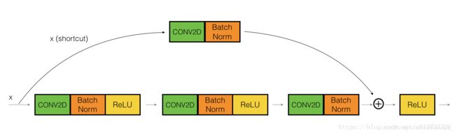
# 恒等块:适用于输入输出维度一致的情况
def identity_block(X, f, filters, stage, block):
    """
    实现恒等块
    :param X:   -输入的tensor类型的数据，维度为(m, n_H_prev, n_W_prev, n_c_prev)
    :param f:   -整数，指定主路径中间的CONV窗口的维度
    :param filters: -整数列表，定义了主路径每层的卷积层的过滤器数量
    :param stage:   -整数，根据每层的位置来命名每一层，与block参数一起使用
    :param block:   -字符串，根据每层的位置来命名每一层，与stage参数一起使用
    :return: X      -恒等块的输出，tensor类型，维度为(n_H, n_W, n_c)
    """

    # 定义命名规则
    conv_name_base = "res" + str(stage) + block + "_branch"
    bn_name_base = "bn" + str(stage) + block + "_branch"

    # 获取过滤器
    F1, F2, F3 = filters

    # 保存输入数据，将会用于为主路径添加捷径
    X_shortcut = X

    # 主路径的第一部分
    ## 卷积层
    X = Conv2D(filters=F1, kernel_size=(1, 1), strides=(1, 1), padding="valid",
               name=conv_name_base+"2a", kernel_initializer=glorot_uniform(seed=0))(X)

    ## 归一化
    X = BatchNormalization(axis=3, name=bn_name_base+"2a")(X)
    ## 使用ReLU激活函数
    X = Activation("relu")(X)

    # 主路径的第二部分
    ## 卷积层
    X = Conv2D(filters=F2, kernel_size=(f, f), strides=(1, 1), padding="same",
               name=conv_name_base + "2b", kernel_initializer=glorot_uniform(seed=0))(X)

    ## 归一化
    X = BatchNormalization(axis=3, name=bn_name_base + "2b")(X)
    ## 使用ReLU激活函数
    X = Activation("relu")(X)

    # 主路径的第三部分
    ## 卷积层
    X = Conv2D(filters=F3, kernel_size=(1, 1), strides=(1, 1), padding="valid",
               name=conv_name_base + "2c", kernel_initializer=glorot_uniform(seed=0))(X)

    ## 归一化
    X = BatchNormalization(axis=3, name=bn_name_base + "2c")(X)
    ## 没有ReLU激活函数

    # 最后一步：
    ## 将捷径与输入加在一起
    X = Add()([X, X_shortcut])
    ## 使用ReLU激活函数
    X = Activation("relu")(X)

    return X

print("=========================测试identity_block=======================")
# tf.compat.v1.reset_defult_graph()
# tf.compat.v1.disable_eager_execution()
test = tf.compat.v1.Session()
with tf.compat.v1.Session() as test:
    np.random.seed(1)
    A_prev = tf.compat.v1.placeholder("float", [3, 4, 4, 6])
    X = np.random.randn(3, 4, 4, 6)
    A = identity_block(A_prev, f=2, filters=[2, 4, 6], stage=1, block="a")

    test.run(tf.compat.v1.global_variables_initializer())
    out = test.run([A], feed_dict={A_prev: X, K.learning_phase(): 0})
    print("out = " + str(out[0][1][1][0]))      # out = [0.        0.        1.3454674 2.031818  0.        1.3246754]

    test.close()


# 卷积块：适用于输入输出维度不一致的情况
def convolutional_block(X, f, filters, stage, block, s=2):
    """
    实现卷积块
    :param X:   -输入的tensor类型的数据，维度为(m, n_H_prev, n_W_prev, n_c_prev)
    :param f:   -整数，指定主路径中间的CONV窗口的维度
    :param filters: -整数列表，定义了主路径每层的卷积层的过滤器数量
    :param stage:   -整数，根据每层的位置来命名每一层，与block参数一起使用
    :param block:   -字符串，根据每层的位置来命名每一层，与stage参数一起使用
    :param s:       -整数，指定要使用的步幅
    :return: X      -卷积块的输出，tensor类型，维度为(n_H, n_W, n_c)
    """

    # 定义命名规则
    conv_name_base = "res" + str(stage) + block + "_branch"
    bn_name_base = "bn" + str(stage) + block + "_branch"

    # 获取过滤器
    F1, F2, F3 = filters

    # 保存输入数据，将会用于为主路径添加捷径
    X_shortcut = X

    # 主路径
    ## 主路径的第一部分
    X = Conv2D(filters=F1, kernel_size=(1, 1), strides=(s, s), padding="valid",
               name=conv_name_base+"2a", kernel_initializer=glorot_uniform(seed=0))(X)
    X = BatchNormalization(axis=3, name=bn_name_base+"2a")(X)
    X = Activation("relu")(X)

    ## 主路径的第二部分
    X = Conv2D(filters=F2, kernel_size=(f, f), strides=(1, 1), padding="same",
               name=conv_name_base + "2b", kernel_initializer=glorot_uniform(seed=0))(X)
    X = BatchNormalization(axis=3, name=bn_name_base + "2b")(X)
    X = Activation("relu")(X)

    ## 主路径的第三部分
    X = Conv2D(filters=F3, kernel_size=(1, 1), strides=(1, 1), padding="valid",
               name=conv_name_base + "2c", kernel_initializer=glorot_uniform(seed=0))(X)
    X = BatchNormalization(axis=3, name=bn_name_base + "2c")(X)


    # 捷径
    X_shortcut = Conv2D(filters=F3, kernel_size=(1, 1), strides=(s, s), padding="valid",
                        name=conv_name_base+"1", kernel_initializer=glorot_uniform(seed=0))(X_shortcut)
    X_shortcut = BatchNormalization(axis=3, name=bn_name_base+"1")(X_shortcut)


    # 最后一步：
    ## 将捷径与输入加在一起
    X = Add()([X, X_shortcut])
    ## 使用ReLU激活函数
    X = Activation("relu")(X)

    return X

print("=========================测试convolutional_block=======================")
# tf.compat.v1.reset_defult_graph()
# tf.compat.v1.disable_eager_execution()
test = tf.compat.v1.Session()
with tf.compat.v1.Session() as test:
    np.random.seed(1)
    A_prev = tf.compat.v1.placeholder("float", [3, 4, 4, 6])
    X = np.random.randn(3, 4, 4, 6)
    A = convolutional_block(A_prev, f=2, filters=[2, 4, 6], stage=1, block="a")

    test.run(tf.compat.v1.global_variables_initializer())
    out = test.run([A], feed_dict={A_prev: X, K.learning_phase(): 0})
    print("out = " + str(out[0][1][1][0]))  # out = [0.         0.         0.         0.8929657  0.         0.19882731]

    test.close()


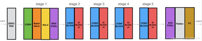
# 构建残差网络(50层)
def ResNet50(input_shape=(64, 64, 3), classes=6):
    """
    实现ResNet50
        CONV2D -> BATCHNORM -> RELU -> MAXPOOL -> CONVBLOCK -> IDBLOCK*2 -> CONVBLOCK -> IDBLOCK*3
        -> CONVBLOCK -> IDBLOCK*5 -> CONVBLOCK -> IDBLOCK*2 -> AVGPOOL -> TOPLAYER
    :param input_shape:     -图像数据集的维度
    :param classes:         -整数，分类数
    :return: model          -Keras框架的模型
    """

    # 定义tensor类型的输入数据
    X_input = Input(input_shape)

    # 0填充
    X = ZeroPadding2D((3, 3))(X_input)
    print(X.shape)  # (None, 70, 70, 3)

    # stage1
    X = Conv2D(filters=64, kernel_size=(7, 7), strides=(2, 2), name="conv1",
               kernel_initializer=glorot_uniform(seed=0))(X)
    X = BatchNormalization(axis=3, name="bn_conv1")(X)
    X = Activation("relu")(X)
    X = MaxPooling2D(pool_size=(3, 3), strides=(2, 2))(X)
    print(X.shape)  # (None, 15, 15, 64)

    # stage2
    X = convolutional_block(X, f=3, filters=[64, 64, 256], stage=2, block="a", s=1)
    X = identity_block(X, f=3, filters=[64, 64, 256], stage=2, block="b")
    X = identity_block(X, f=3, filters=[64, 64, 256], stage=2, block="c")
    print(X.shape)  # (None, 15, 15, 256)

    # stage3
    X = convolutional_block(X, f=3, filters=[128, 128, 512], stage=3, block="a", s=2)
    X = identity_block(X, f=3, filters=[128, 128, 512], stage=3, block="b")
    X = identity_block(X, f=3, filters=[128, 128, 512], stage=3, block="c")
    X = identity_block(X, f=3, filters=[128, 128, 512], stage=3, block="d")
    print(X.shape)  # (None, 8, 8, 512)

    # stage4
    X = convolutional_block(X, f=3, filters=[256, 256, 1024], stage=4, block="a", s=2)
    X = identity_block(X, f=3, filters=[256, 256, 1024], stage=4, block="b")
    X = identity_block(X, f=3, filters=[256, 256, 1024], stage=4, block="c")
    X = identity_block(X, f=3, filters=[256, 256, 1024], stage=4, block="d")
    X = identity_block(X, f=3, filters=[256, 256, 1024], stage=4, block="e")
    X = identity_block(X, f=3, filters=[256, 256, 1024], stage=4, block="f")
    print(X.shape)  # (None, 4, 4, 1024)

    # stage5
    X = convolutional_block(X, f=3, filters=[512, 512, 2048], stage=5, block="a", s=2)
    X = identity_block(X, f=3, filters=[512, 512, 2048], stage=5, block="b")
    X = identity_block(X, f=3, filters=[512, 512, 2048], stage=5, block="c")
    print(X.shape)  # (None, 2, 2, 2048)

    # 均值池化层
    X = AveragePooling2D(pool_size=(2, 2), padding="same")(X)
    print(X.shape)  # (None, 1, 1, 2048)

    # 输出层
    X = Flatten()(X)
    print(X.shape)  # (None, 2048)
    X = Dense(classes, activation="softmax", name="fc"+str(classes),
              kernel_initializer=glorot_uniform(seed=0))(X)
    print(X.shape)  # (None, 6)


    # 创建模型
    model = Model(inputs=X_input, outputs=X, name="ResNet50")

    return model

# 对模型实体化和编译
model = ResNet50(input_shape=(64, 64, 3), classes=6)
model.compile(optimizer="adam", loss="categorical_crossentropy", metrics=["accuracy"])



# 加载数据集，数据集同test2_3
X_train_orig, Y_train_orig, X_test_orig, Y_test_orig, classes = Deep_Learning.test4_2.resnets_utils.load_dataset()
index = 6
plt.imshow(X_train_orig[index])
plt.show()
print("Y = " + str(np.squeeze(Y_train_orig[:, index])))     # Y = 2

# Normalize image vectors
X_train = X_train_orig / 255
X_test = X_test_orig / 255

# Covert training and test labels to one hot matrices
Y_train = Deep_Learning.test4_2.resnets_utils.convert_to_one_hot(Y_train_orig, 6).T
Y_test = Deep_Learning.test4_2.resnets_utils.convert_to_one_hot(Y_test_orig, 6).T

print("训练集样本数 = " + str(X_train.shape[0]))                  # 训练集样本数 = 1080
print("测试集样本数 = " + str(X_test.shape[0]))                   # 测试集样本数 = 120
print("X_train.shape:" + str(X_train.shape))                    # X_train.shape:(1080, 64, 64, 3)
print("Y_train.shape:" + str(Y_train.shape))                    # Y_train.shape:(1080, 6)
print("X_test.shape:" + str(X_test.shape))                      # X_test.shape:(120, 64, 64, 3)
print("Y_test.shape:" + str(Y_test.shape))                      # Y_test.shape:(120, 6)


# 运行模型两代，batch=32，每代约3min
model.fit(X_train, Y_train, epochs=2, batch_size=32)

# 评估模型
preds = model.evaluate(X_test, Y_test)
print("误差值 = " + str(preds[0]))
print("准确率 = " + str(preds[1]))
"""
    运行结果：
        Epoch 1/2
        34/34 [==============================] - 90s 3s/step - loss: 2.1543 - accuracy: 0.4694
        Epoch 2/2
        34/34 [==============================] - 88s 3s/step - loss: 0.7385 - accuracy: 0.7463
        4/4 [==============================] - 0s 123ms/step - loss: 5.0244 - accuracy: 0.1667
        误差值 = 5.024357318878174
        准确率 = 0.1666666716337204
"""


"""
    继续训练RESNET20代时，能得到更好的性能，但在CPU上训练需要一个多小时。
    使用GPU的话博主已经在手势数据集上训练了自己的RESNET50模型的权重，可以直接运行博主的训练模型，加载模型可能需要1min。
"""
model = load_model("ResNet50.h5")
preds = model.evaluate(X_test, Y_test)
print("误差值 = " + str(preds[0]))
print("准确率 = " + str(preds[1]))
"""
    运行结果：
        4/4 [==============================] - 0s 121ms/step - loss: 0.1085 - accuracy: 0.9667
        误差值 = 0.1085430383682251
        准确率 = 0.9666666388511658
"""



# 使用自己的图片测试
img_path = 'images/fingers_2.jpg'

my_image = image.load_img(img_path, target_size=(64, 64))
my_image = image.img_to_array(my_image)

my_image = np.expand_dims(my_image, axis=0) / 255
my_image = preprocess_input(my_image)

print("my_image.shape = " + str(my_image.shape))
print("class prediction vector [p(0), p(1), p(2), p(3), p(4), p(5) = ")
print(model.predict(my_image))
"""
    运行结果：(结果不正确)
        my_image.shape = (1, 64, 64, 3)
        class prediction vector [p(0), p(1), p(2), p(3), p(4), p(5) = 
        [[1. 0. 0. 0. 0. 0.]]
"""

# my_image = scipy.misc.imread(img_path)  # module 'scipy.misc' has no attribute 'imread'
my_image = imageio.imread(img_path)
plt.imshow(my_image)
plt.show()


# 查看网络节点的大小细节
model.summary()


# 绘制结构图
plot_model(model, to_file='model.png')
SVG(model_to_dot(model).create(prog='dot', format='svg'))

恒等块

卷积块

ResNet-50

运行结果

Model: "ResNet50"
__________________________________________________________________________________________________
Layer (type)                    Output Shape         Param #     Connected to                     
==================================================================================================
input_1 (InputLayer)            [(None, 64, 64, 3)]  0                                            
__________________________________________________________________________________________________
zero_padding2d_1 (ZeroPadding2D (None, 70, 70, 3)    0           input_1[0][0]                    
__________________________________________________________________________________________________
conv1 (Conv2D)                  (None, 32, 32, 64)   9472        zero_padding2d_1[0][0]           
__________________________________________________________________________________________________
bn_conv1 (BatchNormalization)   (None, 32, 32, 64)   256         conv1[0][0]                      
__________________________________________________________________________________________________
activation_1 (Activation)       (None, 32, 32, 64)   0           bn_conv1[0][0]                   
__________________________________________________________________________________________________
max_pooling2d_1 (MaxPooling2D)  (None, 15, 15, 64)   0           activation_1[0][0]               
__________________________________________________________________________________________________
......
Total params: 23,600,006
Trainable params: 23,546,886
Non-trainable params: 53,120
__________________________________________________________________________________________________

resnet_utils.py

import os
import numpy as np
import tensorflow as tf
import h5py
import math

def load_dataset():
    train_dataset = h5py.File('datasets/train_signs.h5', "r")
    train_set_x_orig = np.array(train_dataset["train_set_x"][:]) # your train set features
    train_set_y_orig = np.array(train_dataset["train_set_y"][:]) # your train set labels

    test_dataset = h5py.File('datasets/test_signs.h5', "r")
    test_set_x_orig = np.array(test_dataset["test_set_x"][:]) # your test set features
    test_set_y_orig = np.array(test_dataset["test_set_y"][:]) # your test set labels

    classes = np.array(test_dataset["list_classes"][:]) # the list of classes
    
    train_set_y_orig = train_set_y_orig.reshape((1, train_set_y_orig.shape[0]))
    test_set_y_orig = test_set_y_orig.reshape((1, test_set_y_orig.shape[0]))
    
    return train_set_x_orig, train_set_y_orig, test_set_x_orig, test_set_y_orig, classes


def random_mini_batches(X, Y, mini_batch_size = 64, seed = 0):
    """
    Creates a list of random minibatches from (X, Y)
    
    Arguments:
    X -- input data, of shape (input size, number of examples) (m, Hi, Wi, Ci)
    Y -- true "label" vector (containing 0 if cat, 1 if non-cat), of shape (1, number of examples) (m, n_y)
    mini_batch_size - size of the mini-batches, integer
    seed -- this is only for the purpose of grading, so that you're "random minibatches are the same as ours.
    
    Returns:
    mini_batches -- list of synchronous (mini_batch_X, mini_batch_Y)
    """
    
    m = X.shape[0]                  # number of training examples
    mini_batches = []
    np.random.seed(seed)
    
    # Step 1: Shuffle (X, Y)
    permutation = list(np.random.permutation(m))
    shuffled_X = X[permutation,:,:,:]
    shuffled_Y = Y[permutation,:]

    # Step 2: Partition (shuffled_X, shuffled_Y). Minus the end case.
    num_complete_minibatches = math.floor(m/mini_batch_size) # number of mini batches of size mini_batch_size in your partitionning
    for k in range(0, num_complete_minibatches):
        mini_batch_X = shuffled_X[k * mini_batch_size : k * mini_batch_size + mini_batch_size,:,:,:]
        mini_batch_Y = shuffled_Y[k * mini_batch_size : k * mini_batch_size + mini_batch_size,:]
        mini_batch = (mini_batch_X, mini_batch_Y)
        mini_batches.append(mini_batch)
    
    # Handling the end case (last mini-batch < mini_batch_size)
    if m % mini_batch_size != 0:
        mini_batch_X = shuffled_X[num_complete_minibatches * mini_batch_size : m,:,:,:]
        mini_batch_Y = shuffled_Y[num_complete_minibatches * mini_batch_size : m,:]
        mini_batch = (mini_batch_X, mini_batch_Y)
        mini_batches.append(mini_batch)
    
    return mini_batches


def convert_to_one_hot(Y, C):
    Y = np.eye(C)[Y.reshape(-1)].T
    return Y


def forward_propagation_for_predict(X, parameters):
    """
    Implements the forward propagation for the model: LINEAR -> RELU -> LINEAR -> RELU -> LINEAR -> SOFTMAX
    
    Arguments:
    X -- input dataset placeholder, of shape (input size, number of examples)
    parameters -- python dictionary containing your parameters "W1", "b1", "W2", "b2", "W3", "b3"
                  the shapes are given in initialize_parameters
    Returns:
    Z3 -- the output of the last LINEAR unit
    """
    
    # Retrieve the parameters from the dictionary "parameters" 
    W1 = parameters['W1']
    b1 = parameters['b1']
    W2 = parameters['W2']
    b2 = parameters['b2']
    W3 = parameters['W3']
    b3 = parameters['b3'] 
                                                           # Numpy Equivalents:
    Z1 = tf.add(tf.matmul(W1, X), b1)                      # Z1 = np.dot(W1, X) + b1
    A1 = tf.nn.relu(Z1)                                    # A1 = relu(Z1)
    Z2 = tf.add(tf.matmul(W2, A1), b2)                     # Z2 = np.dot(W2, a1) + b2
    A2 = tf.nn.relu(Z2)                                    # A2 = relu(Z2)
    Z3 = tf.add(tf.matmul(W3, A2), b3)                     # Z3 = np.dot(W3,Z2) + b3
    
    return Z3

def predict(X, parameters):
    
    W1 = tf.convert_to_tensor(parameters["W1"])
    b1 = tf.convert_to_tensor(parameters["b1"])
    W2 = tf.convert_to_tensor(parameters["W2"])
    b2 = tf.convert_to_tensor(parameters["b2"])
    W3 = tf.convert_to_tensor(parameters["W3"])
    b3 = tf.convert_to_tensor(parameters["b3"])
    
    params = {"W1": W1,
              "b1": b1,
              "W2": W2,
              "b2": b2,
              "W3": W3,
              "b3": b3}
    
    x = tf.placeholder("float", [12288, 1])
    
    z3 = forward_propagation_for_predict(x, params)
    p = tf.argmax(z3)
    
    sess = tf.Session()
    prediction = sess.run(p, feed_dict = {x: X})
        
    return prediction