带有Python的AI –分析时间序列数据

带有Python的AI –分析时间序列数据 (AI with Python – Analyzing Time Series Data)

Predicting the next in a given input sequence is another important concept in machine learning. This chapter gives you a detailed explanation about analyzing time series data.

预测给定输入序列中的下一个是机器学习中的另一个重要概念。 本章为您提供有关分析时间序列数据的详细说明。

介绍 (Introduction)

Time series data means the data that is in a series of particular time intervals. If we want to build sequence prediction in machine learning, then we have to deal with sequential data and time. Series data is an abstract of sequential data. Ordering of data is an important feature of sequential data.

时间序列数据是指一系列特定时间间隔中的数据。 如果我们想在机器学习中建立序列预测，那么我们必须处理顺序数据和时间。 系列数据是顺序数据的抽象。 数据排序是顺序数据的重要特征。

序列分析或时间序列分析的基本概念 (Basic Concept of Sequence Analysis or Time Series Analysis)

Sequence analysis or time series analysis is to predict the next in a given input sequence based on the previously observed. The prediction can be of anything that may come next: a symbol, a number, next day weather, next term in speech etc. Sequence analysis can be very handy in applications such as stock market analysis, weather forecasting, and product recommendations.

序列分析或时间序列分析是基于先前观察到的预测给定输入序列中的下一个序列。 预测可以是接下来可能发生的任何事情：符号，数字，第二天的天气，下一个言语等。序列分析在诸如股票市场分析，天气预报和产品推荐之类的应用中非常方便。

Example

例

Consider the following example to understand sequence prediction. Here A,B,C,D are the given values and you have to predict the value E using a Sequence Prediction Model.

考虑以下示例以了解序列预测。 在这里， A，B，C，D是给定的值，您必须使用序列预测模型来预测值E。

安装有用的软件包 (Installing Useful Packages)

For time series data analysis using Python, we need to install the following packages −

对于使用Python进行时间序列数据分析，我们需要安装以下软件包-

大熊猫 (Pandas)

Pandas is an open source BSD-licensed library which provides high-performance, ease of data structure usage and data analysis tools for Python. You can install Pandas with the help of the following command −

Pandas是开源的BSD许可库，它为Python提供了高性能，易于使用的数据结构和数据分析工具。 您可以在以下命令的帮助下安装Pandas-

pip install pandas

If you are using Anaconda and want to install by using the conda package manager, then you can use the following command −

如果您正在使用Anaconda并想使用conda软件包管理器进行安装，则可以使用以下命令-

conda install -c anaconda pandas

学习 (hmmlearn)

It is an open source BSD-licensed library which consists of simple algorithms and models to learn Hidden Markov Models(HMM) in Python. You can install it with the help of the following command −

它是开放源代码BSD许可的库，由简单的算法和模型组成，以学习Python中的隐马尔可夫模型(HMM)。 您可以在以下命令的帮助下安装它-

pip install hmmlearn

If you are using Anaconda and want to install by using the conda package manager, then you can use the following command −

如果您正在使用Anaconda并想使用conda软件包管理器进行安装，则可以使用以下命令-

conda install -c omnia hmmlearn

PyStruct (PyStruct)

It is a structured learning and prediction library. Learning algorithms implemented in PyStruct have names such as conditional random fields(CRF), Maximum-Margin Markov Random Networks (M3N) or structural support vector machines. You can install it with the help of the following command −

它是一个结构化的学习和预测库。 在PyStruct中实现的学习算法的名称包括条件随机字段(CRF)，最大边距马尔可夫随机网络(M3N)或结构支持向量机。 您可以在以下命令的帮助下安装它-

pip install pystruct

CVXOPT (CVXOPT)

It is used for convex optimization based on Python programming language. It is also a free software package. You can install it with the help of following command −

它用于基于Python编程语言的凸优化。 它也是一个免费软件包。 您可以在以下命令的帮助下安装它-

pip install cvxopt

If you are using Anaconda and want to install by using the conda package manager, then you can use the following command −

如果您正在使用Anaconda并想使用conda软件包管理器进行安装，则可以使用以下命令-

conda install -c anaconda cvdoxt

熊猫：从时间序列数据中处理，切片和提取统计信息 (Pandas: Handling, Slicing and Extracting Statistic from Time Series Data)

Pandas is a very useful tool if you have to work with time series data. With the help of Pandas, you can perform the following −

如果必须使用时间序列数据，Pandas是非常有用的工具。 借助Pandas，您可以执行以下操作-

• Create a range of dates by using the pd.date_range package

  通过使用pd.date_range包创建日期范围

• Index pandas with dates by using the pd.Series package

  通过使用pd.Series包为熊猫索引日期

• Perform re-sampling by using the ts.resample package

  使用ts.resample包执行重新采样

• Change the frequency

  改变频率

例 (Example)

The following example shows you handling and slicing the time series data by using Pandas. Note that here we are using the Monthly Arctic Oscillation data, which can be downloaded from monthly.ao.index.b50.current.ascii and can be converted to text format for our use.

以下示例显示了使用Pandas处理和切片时间序列数据的方法。 请注意，这里我们使用的是每月北极涛动数据，该数据可以从monthly.ao.index.b50.current.ascii下载，并可以转换为文本格式供我们使用。

处理时间序列数据 (Handling time series data)

For handling time series data, you will have to perform the following steps −

为了处理时间序列数据，您将必须执行以下步骤-

The first step involves importing the following packages −

第一步涉及导入以下软件包-

import numpy as np
import matplotlib.pyplot as plt
import pandas as pd

Next, define a function which will read the data from the input file, as shown in the code given below −

接下来，定义一个将从输入文件中读取数据的函数，如下面的代码所示-

def read_data(input_file):
   input_data = np.loadtxt(input_file, delimiter = None)

Now, convert this data to time series. For this, create the range of dates of our time series. In this example, we keep one month as frequency of data. Our file is having the data which starts from January 1950.

现在，将此数据转换为时间序列。 为此，请创建我们时间序列的日期范围。 在此示例中，我们将一个月作为数据频率。 我们的文件包含的数据始于1950年1月。

dates = pd.date_range('1950-01', periods = input_data.shape[0], freq = 'M')

In this step, we create the time series data with the help of Pandas Series, as shown below −

在此步骤中，我们借助Pandas Series创建时间序列数据，如下所示-

output = pd.Series(input_data[:, index], index = dates)	
return output
	
if __name__=='__main__':

Enter the path of the input file as shown here −

输入输入文件的路径，如下所示-

input_file = "/Users/admin/AO.txt"

Now, convert the column to timeseries format, as shown here −

现在，将列转换为时间序列格式，如下所示：

timeseries = read_data(input_file)

Finally, plot and visualize the data, using the commands shown −

最后，使用所示命令绘制并可视化数据-

plt.figure()
timeseries.plot()
plt.show()

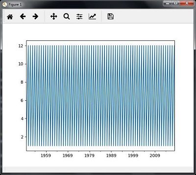
You will observe the plots as shown in the following images −

您将观察到如下图所示的图-

切片时间序列数据 (Slicing time series data)

Slicing involves retrieving only some part of the time series data. As a part of the example, we are slicing the data only from 1980 to 1990. Observe the following code that performs this task −

切片涉及仅检索时间序列数据的一部分。 作为示例的一部分，我们仅对1980年至1990年的数据进行切片。请观察执行此任务的以下代码-

timeseries['1980':'1990'].plot()
   

plt.show()

When you run the code for slicing the time series data, you can observe the following graph as shown in the image here −

当您运行用于对时间序列数据进行切片的代码时，您可以观察到以下图形，如此处的图像所示：

从时间序列数据中提取统计信息 (Extracting Statistic from Time Series Data)

You will have to extract some statistics from a given data, in cases where you need to draw some important conclusion. Mean, variance, correlation, maximum value, and minimum value are some of such statistics. You can use the following code if you want to extract such statistics from a given time series data −

如果需要得出一些重要的结论，则必须从给定的数据中提取一些统计信息。 均值，方差，相关性，最大值和最小值就是这样的统计信息。 如果要从给定的时间序列数据中提取此类统计信息，则可以使用以下代码-

意思 (Mean)

You can use the mean() function, for finding the mean, as shown here −

您可以使用mean()函数来查找均值，如下所示：

timeseries.mean()

Then the output that you will observe for the example discussed is −

那么您将在讨论的示例中观察到的输出是-

-0.11143128165238671

最大值 (Maximum)

You can use the max() function, for finding maximum, as shown here −

您可以使用max()函数来查找最大值，如下所示-

timeseries.max()

Then the output that you will observe for the example discussed is −

那么您将在讨论的示例中观察到的输出是-

3.4952999999999999

最低要求 (Minimum)

You can use the min() function, for finding minimum, as shown here −

您可以使用min()函数来查找最小值，如下所示-

timeseries.min()

Then the output that you will observe for the example discussed is −

那么您将在讨论的示例中观察到的输出是-

-4.2656999999999998

一次获取所有内容 (Getting everything at once)

If you want to calculate all statistics at a time, you can use the describe() function as shown here −

如果您想一次计算所有统计信息，则可以使用describe()函数，如下所示：

timeseries.describe()

Then the output that you will observe for the example discussed is −

那么您将在讨论的示例中观察到的输出是-

count   817.000000
mean     -0.111431
std       1.003151
min      -4.265700
25%      -0.649430
50%      -0.042744
75%       0.475720
max       3.495300
dtype: float64

重采样 (Re-sampling)

You can resample the data to a different time frequency. The two parameters for performing re-sampling are −

您可以将数据重新采样为其他时间频率。 用于执行重采样的两个参数是-

• Time period
  时间段
• Method
  方法

用mean()重新采样 (Re-sampling with mean())

You can use the following code to resample the data with the mean()method, which is the default method −

您可以使用以下代码通过mean()方法对数据进行重新采样，这是默认方法-

timeseries_mm = timeseries.resample("A").mean()
timeseries_mm.plot(style = 'g--')
plt.show()

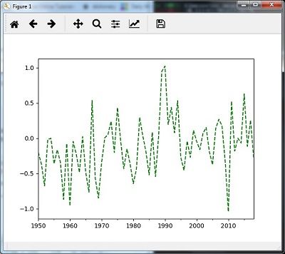
Then, you can observe the following graph as the output of resampling using mean() −

然后，您可以观察下图作为使用mean()重采样的输出-

用中位数()重新采样 (Re-sampling with median())

You can use the following code to resample the data using the median()method −

您可以使用以下代码通过中位数()方法对数据进行重新采样-

timeseries_mm = timeseries.resample("A").median()
timeseries_mm.plot()
plt.show()

Then, you can observe the following graph as the output of re-sampling with median() −

然后，您可以观察到以下图表，作为使用mean()进行重新采样的输出-

滚动平均值 (Rolling Mean)

You can use the following code to calculate the rolling (moving) mean −

您可以使用以下代码来计算滚动(移动)均值-

timeseries.rolling(window = 12, center = False).mean().plot(style = '-g')
plt.show()

Then, you can observe the following graph as the output of the rolling (moving) mean −

然后，您可以观察下图作为滚动(移动)平均值的输出：

通过隐马尔可夫模型(HMM)分析顺序数据 (Analyzing Sequential Data by Hidden Markov Model (HMM))

HMM is a statistic model which is widely used for data having continuation and extensibility such as time series stock market analysis, health checkup, and speech recognition. This section deals in detail with analyzing sequential data using Hidden Markov Model (HMM).

HMM是一种统计模型，广泛用于具有连续性和可扩展性的数据，例如时间序列股票市场分析，健康状况检查和语音识别。 本节详细介绍使用隐马尔可夫模型(HMM)分析顺序数据。

隐马尔可夫模型(HMM) (Hidden Markov Model (HMM))

HMM is a stochastic model which is built upon the concept of Markov chain based on the assumption that probability of future stats depends only on the current process state rather any state that preceded it. For example, when tossing a coin, we cannot say that the result of the fifth toss will be a head. This is because a coin does not have any memory and the next result does not depend on the previous result.

HMM是一种基于马尔可夫链概念的随机模型，该模型基于以下假设：未来统计信息的概率仅取决于当前流程状态，而不取决于其之前的任何状态。 例如，抛硬币时，我们不能说第五次抛的结果是正面。 这是因为硬币没有任何记忆，下一个结果不取决于前一个结果。

Mathematically, HMM consists of the following variables −

从数学上讲，HMM由以下变量组成-

州(S) (States (S))

It is a set of hidden or latent states present in a HMM. It is denoted by S.

它是HMM中存在的一组隐藏或潜在状态。 用S表示。

输出符号(O) (Output symbols (O))

It is a set of possible output symbols present in a HMM. It is denoted by O.

它是HMM中存在的一组可能的输出符号。 用O表示。

状态转移概率矩阵(A) (State Transition Probability Matrix (A))

It is the probability of making transition from one state to each of the other states. It is denoted by A.

这是从一个状态过渡到其他状态的概率。 用A表示。

观测排放概率矩阵(B) (Observation Emission Probability Matrix (B))

It is the probability of emitting/observing a symbol at a particular state. It is denoted by B.

它是在特定状态下发射/观察符号的概率。 用B表示。

先验概率矩阵(Π) (Prior Probability Matrix (Π))

It is the probability of starting at a particular state from various states of the system. It is denoted by Π.

它是从系统的各种状态开始于特定状态的概率。 用表示。

Hence, a HMM may be defined as = (S,O,A,B,),

因此，可以将HMM定义为 =(S，O，A，B，) ，

where,

哪里，

• S = {s₁,s₂,…,s_N} is a set of N possible states,

  S = {s ₁ ，s ₂ ，…，s _N }是N个可能状态的集合，

• O = {o₁,o₂,…,o_M} is a set of M possible observation symbols,

  O = {o ₁ ，o ₂ ，…，o _M }是一组M个可能的观测符号，

• A is an NN state Transition Probability Matrix (TPM),

  A是NN状态转移概率矩阵(TPM)，

• B is an NM observation or Emission Probability Matrix (EPM),

  B是NM观测或发射概率矩阵(EPM)，

• π is an N dimensional initial state probability distribution vector.
  π是N维初始状态概率分布矢量。

示例：股票市场数据分析 (Example: Analysis of Stock Market data)

In this example, we are going to analyze the data of stock market, step by step, to get an idea about how the HMM works with sequential or time series data. Please note that we are implementing this example in Python.

在此示例中，我们将逐步分析股票市场数据，以了解HMM如何处理顺序数据或时间序列数据。 请注意，我们正在用Python实现此示例。

Import the necessary packages as shown below −

导入必要的软件包，如下所示：

import datetime
import warnings

Now, use the stock market data from the matpotlib.finance package, as shown here −

现在，使用matpotlib.finance包中的股市数据，如下所示-

import numpy as np
from matplotlib import cm, pyplot as plt
from matplotlib.dates import YearLocator, MonthLocator
try:
   from matplotlib.finance import quotes_historical_yahoo_och1
except ImportError:
   from matplotlib.finance import (
      quotes_historical_yahoo as quotes_historical_yahoo_och1)

from hmmlearn.hmm import GaussianHMM

Load the data from a start date and end date, i.e., between two specific dates as shown here −

从开始日期和结束日期(即两个特定日期之间)加载数据，如下所示-

start_date = datetime.date(1995, 10, 10)
end_date = datetime.date(2015, 4, 25)
quotes = quotes_historical_yahoo_och1('INTC', start_date, end_date)

In this step, we will extract the closing quotes every day. For this, use the following command −

在这一步中，我们将每天提取结束报价。 为此，请使用以下命令-

closing_quotes = np.array([quote[2] for quote in quotes])

Now, we will extract the volume of shares traded every day. For this, use the following command −

现在，我们将提取每天交易的股票数量。 为此，请使用以下命令-

volumes = np.array([quote[5] for quote in quotes])[1:]

Here, take the percentage difference of closing stock prices, using the code shown below −

在这里，使用下面显示的代码来计算收盘价的百分比差-

diff_percentages = 100.0 * np.diff(closing_quotes) / closing_quotes[:-]
dates = np.array([quote[0] for quote in quotes], dtype = np.int)[1:]
training_data = np.column_stack([diff_percentages, volumes])

In this step, create and train the Gaussian HMM. For this, use the following code −

在此步骤中，创建并训练高斯HMM。 为此，请使用以下代码-

hmm = GaussianHMM(n_components = 7, covariance_type = 'diag', n_iter = 1000)
with warnings.catch_warnings():
   warnings.simplefilter('ignore')
   hmm.fit(training_data)

Now, generate data using the HMM model, using the commands shown −

现在，使用所示的命令，使用HMM模型生成数据-

num_samples = 300
samples, _ = hmm.sample(num_samples)

Finally, in this step, we plot and visualize the difference percentage and volume of shares traded as output in the form of graph.

最后，在此步骤中，我们以图表形式绘制并可视化作为输出的交易股票的差异百分比和数量。

Use the following code to plot and visualize the difference percentages −

使用以下代码来绘制和可视化差异百分比-

plt.figure()
plt.title('Difference percentages')
plt.plot(np.arange(num_samples), samples[:, 0], c = 'black')

Use the following code to plot and visualize the volume of shares traded −

使用以下代码来绘制和可视化交易的股票数量-

plt.figure()
plt.title('Volume of shares')
plt.plot(np.arange(num_samples), samples[:, 1], c = 'black')
plt.ylim(ymin = 0)
plt.show()

翻译自: https://www.tutorialspoint.com/artificial_intelligence_with_python/artificial_intelligence_with_python_analyzing_time_series_data.htm