【论文翻译】（五六部分）The Fourier decomposition method for nonlinear and non-stationary time series analysis

5. Simulation and numerical results
5. 模拟和数值结果

Matlab software of the MEMD (http://www.commsp.ee.ic.ac.uk/∼mandic/research/emd.htm), EMD and EEMD (http://rcada.ncu.edu.tw/research1.htm), available online, has been used for simulation results. The objectives of the simulations are (i) to compare the results obtained by the decomposition of signals (widely used in the literature) from the proposed algorithms as well as from the EMD, EEMD and MEMD algorithms; (ii) to demonstrate the efficacy of the proposed FDM for the TFE distribution analysis of simulated as well as reallife (such as earthquake and speech) signals, and compare results with the EMD, EEMD and wavelet transform; (iii) to show that the proposed FDM, like EMD, is not limited by the uncertainty principle. In order to prove the last point, we use the unit sample sequence, which is concentrated in time, and by the proposed method we show that it is also concentrated in frequency. A Matlab code of the proposed FDM has been made publicly available at (https://www.researchgate.net/publication/274570245_Matlab_Code_Of_The_Fourier_Decomposition_Method_FDM).

MEMD (http://www.commsp.ee.ic.ac.uk/∼mandic/research/emd.htm)，EMD and EEMD (http://rcada.ncu.edu.tw/research1.htm)的MATLAB 程序在线可用，已经被用于仿真结果。
仿真的目的是：
(i) 比较本文提出的算法和EMD、EEMD、MEMD算法对信号(文献中广泛使用)进行分解得到的结果；
(ii) 验证所提出的FDM对模拟和现实(如地震和语音)信号的TFE分布分析的有效性，并与EMD、EEMD和小波变换的结果进行比较；
(iii) 证明所提出的FDM像经验模态分解一样，不受不确定性原理的限制。
为了证明最后一点，我们使用了集中在时间上的单位样本序列，并通过所提出的方法证明了它也集中在频率上。所提出的FDM的Matlab代码已在以下网站公开(https://www.researchgate.net/publication/274570245_Matlab_Code_Of_The_Fourier_Decomposition_Method_FDM)。

(a) Intermittency and mode mixing
(a)间歇和模式混合

The intermittency in the time series is a main cause of mode mixing, as shown for signal $x(t)$ in figure 1a, and mode splitting in the EMD algorithm [10]. These issues are mitigated by EEMD and NA-MEMD. The decomposition of a signal $x(t)$ through the FDM algorithm is shown in figure 1b without end effect artefacts. The EMD and EEMD generate 10 IMFs ($y_1$ to $y_{10}$), FDM yields seven FIBFs ($y_1$ to $y_7$), where the sum of $y_1$ to $y_3$, $y_4$ to $y_5$, $y_6$ to $y_{10}$ is represented by $y_1–y_3,y_4–y_5$ and $y_6–y_{10}$, respectively . The FDM is able to localize the mono-component sinusoid within a single FIBF, outperforming the EMD (figure 1c) and EEMD (figure 1d) in terms of reconstruction error, end effect artefacts and orthogonalilty of generated components. On the same machine (Intel core i3 CPU 530 @ 2.93 GHz), the computation time for FDM, EMD and EEMD are 0.56 s, 0.21 s and 77.18 s, respectively . The ensemble size for EEMD was 500 with a 16.94 dB signal-to-noise ratio.

时间序列中的间歇性是模式混合的主要原因，如图1a中的信号 $x(t)$ 和EMD算法中的模式分裂[10]所示。EEMD 和 NA-MEMD 缓解了这些问题。通过FDM对信号 $x(t)$ 进行分解如图 1b所示，没有末端效应伪像。EMD 和 EEMD 产生10个IMFs ($y_1$ 到 $y_{10}$)，FDM 产生7个 FIBFs ($y_1$ 到 $y_7$)， 其中 $y_1$ 到 $y_3$，$y_4$ 到 $y_5$， $y_6$ 到 $y_{10}$ 的和分别展示在图中 $y_1–y_3,y_4–y_5$ 和 $y_6–y_{10}$ 。FDM能够在单个FIBF内定位单分量正弦信号，在重构误差、末端效应伪像和生成分量的正交性方面优于EMD(图1c)和EEMD(图1d)。在相同的机器 (Intel core i3 CPU 530 @ 2.93 GHz)上，FDM, EMD 和 EEMD 的运行时间分别为 0.56 s, 0.21 s 和 77.18 s 。EEMD的总体规模为500，信噪比为16.94 dB。

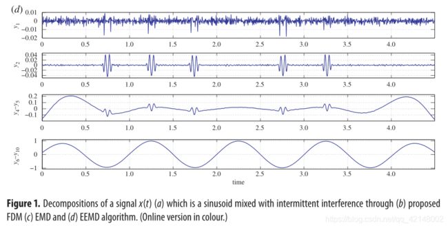
图片1.信号 $x(t)$ 的分解（a）混合了间歇性干扰的正弦信号（b）FDM（c）EMD（d）EEMD算法

(b) Multivariate data decomposition
(b)多元数据分解

We have used quadri-variate time series signal, which is a summation of sinusoids (with combination of frequencies $f_1=4Hz,f_2=8Hz,f_3=16Hz,f_4=32Hz$) and Gaussian white noise with zero mean and standard deviation of 0.2, that is $x_j(t)={\sum }_{i=1}^{4}sin(2\pi f_{i}t)+n_j(t)$ (for $j=1,...,4$). The 32 Hz sinusoid is present in the first, second and fourth channels; the 16 Hz sinusoid is present in the first, second and third channels; the 8 Hz sinusoid is common to all channels; the 4 Hz sinusoid is present in the first, third and fourth channels. On the same machine (Intel core i3 CPU 530 @ 2.93GHz), the computation time for MFDM is 0.45s and for MEMD is 69.5s in this simulation. The MFDM algorithm, similar to MEMD, generates perfectly aligned intrinsic bands, as is clear from the figure 2, in all the four channels, whereas MFDM is computationally more efficient.

我们使用四变量时间序列信号，它是一个正弦信号 (组合频率 $f_1=4Hz,f_2=8Hz,f_3=16Hz,f_4=32Hz$) 和均值为零、标准差为0.2的高斯白噪声的总和，即 $x_j(t)={\sum }_{i=1}^{4}sin(2\pi f_{i}t)+n_j(t)$ ( $j=1,...,4$ )。32 Hz 的正弦波存在于一二四通道；16 Hz 的正弦波存在于一二三通道； 8 Hz 的正弦波存在于所有通道；4 Hz 的正弦波存在于一三四通道。在同样的机器上 (Intel core i3 CPU 530 @ 2.93GHz)，这个仿真MFDM 的计算时间是 0.45s ，MEMD 的计算时间为 69.5s 。从图2中可以清楚的看到，与MEMD类似，MFDM算法在所有四个通道中生成完全对齐的本征频带，而MFDM的计算效率更高。

图2. 将MFDM应用于四变量音调-噪声混合(顶行)，在所有四个通道(第4到第7行)中产生完美对齐的本征模态；第二和第三行包含噪声成分。

（c）Time–frequency–energy analysis of mixture of linear chirp and frequency modulated sinusoid
（c）线性chirp（线性调频信号）和调频正弦混合信号的时-频-能量分析

Figure 3 shows TFE estimates for a non-stationary signal, which is a mixture of a linear chirp and FM sinusoid, obtained using the FDM and EMD algorithm. There is an enhanced TFE tracking when using FDM with LTH-FS. However, the TFE result with HTL-FS is similar to that obtained with EMD algorithm, as can be seen from figure 3.

图3显示了使用FDM和EMD（经验模态分解）算法获得的非平稳信号的TFE估计，该信号是线性chirp和调频正弦波的混合。当使用FDM的LTH-FS时，有一个增强的TFE跟踪。然而，从图3中可以看出，使用HTL-FS的TFE结果类似于使用EMD（经验模态分解）算法获得的结果。

图3. 线性chirp和调频正弦波的混合非平稳信号的TFE分析：(a)(b) FDM （C） EMD

(d) Intrawave frequency modulation
(d) 波内频率调制

We first decompose the following signal that has intrawave frequency modulation and it is considered challenging because the IF itself has very high frequency modulation [33]
$$x(t)=\frac{1}{1.2+\cos (2\pi t)}+\frac{\cos (32\pi t+0.2\cos (64\pi t))}{1.5+\sin (2\pi t)}(5.1)$$

我们首先分解以下具有波内频率调制的信号，这被认为是具有挑战性的，因为IF（瞬时频率）本身具有非常高的频率调制[33]
$$x(t)=\frac{1}{1.2+\cos (2\pi t)}+\frac{\cos (32\pi t+0.2\cos (64\pi t))}{1.5+\sin (2\pi t)}(5.1)$$

Next, we consider a model wave
$$x(t)=\cos (\omega t+ϵ\sin \omega t)(5.2)$$
that satisfies the following highly nonlinear differential equation [3]
$$\frac{d^{2}x(t)}{d{t}^2}+[\omega +ϵ\omega \cos (\omega t){]}^{2}x(t)-[ϵ{\omega }^2\sin (\omega t)]\sqrt{1-x^2(t)}=0(5.3)$$
with $\omega =1$ and $ϵ=0.5$. We demonstrate through figures 4–7 that our method applies well to these challenging cases with good accuracy . For input signal (5.1), FDM yields two FIBFs and TFE distribution without end effects; however, EMD generates three IMFs and TFE distribution has end effects (figure 6). The main difference between the performance of the FDM and the EMD algorithm, for signal (5.2), is the end effects (figure 7). Moreover, both methods are able to reveal intrawave frequency modulation and nonlinearity present in the signals. These examples clearly demonstrate that the proposed FDM can indeed be applied for the analysis of nonlinear signals.

接下来，我们考虑一个模型波
$$x(t)=\cos (\omega t+ϵ\sin \omega t)(5.2)$$
满足以下高度非线性微分方程[3]
$$\frac{d^{2}x(t)}{d{t}^2}+[\omega +ϵ\omega \cos (\omega t){]}^{2}x(t)-[ϵ{\omega }^2\sin (\omega t)]\sqrt{1-x^2(t)}=0(5.3)$$
其中 $\omega =1$ ， $ϵ=0.5$。我们通过图4-7证明了我们的方法可以很好地应用于这些具有挑战性的案例，并具有良好的准确性。对于输入信号(5.1)，FDM产生两个FIBFs，且TFE分布没有末端效应；然而，EMD产生三个IMFs，且TFE分布具有末端效应(图6)。对于信号(5.2)，FDM和EMD算法的性能的主要区别是末端效应(图7)。此外，两种方法都能够揭示信号中存在的波内调频和非线性。这些例子清楚地说明了所提出的FDM确实可以应用于非线性信号的分析。

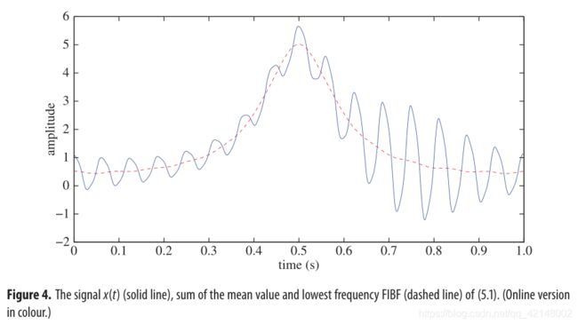
图4. 信号（5.1）：信号$x(t)$（实线），平均值和最低频率FIBF之和(虚线)。

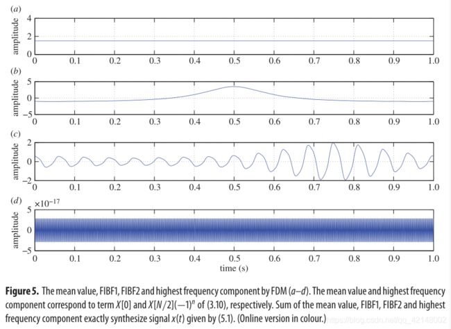
图5. 平均值、FIBF1、FIBF2和FDM的最高频率分量(a–d)。其平均值和最高频率分量分别对应于（3.10）的$X[0]$和X[N/2] (−1)^n$。均值、FIBF1、FIBF2和最高频率分量的和精确合成了(5.1)给出的信号 $x(t)$ 。

图6. 由(5.1)给出的信号 $x(t)$ 的TFE分析：(a) FDM，(b) EMD。注意EMD在TFE图中的末端效应。

图7. 由(5.2)给出的信号 $x(t)$ 的TFE分析：(a) FDM，(b) EMD。注意EMD在TFE图中的末端效应。

(e) Analysis of a white Gaussian noise
(e) 高斯白噪声的分析

Figure 8 shows the TFE analysis of a white Gaussian noise (with zero mean, unit variance, 1024 samples and sampling frequency $F_s$=100 Hz) obtained from the FDM and EMD algorithm. Clearly , both LTH-FS and HTL-FS views of TFE are similar and the entire data are decomposed into a set of FIBFs of distinct frequency bands. Figure 9 shows the power spectral density (PSD) plot of the same white Gaussian noise with the FDM and the EMD algorithm. The FDM has decomposed the entire data into narrowband and orthogonal FIBFs; however, EMD is unable to separate the bands and there is severe energy leakage among the IMFs. Both LTH-FS and HTL-FS views of PSD look similar but FIBFs have different frequency bands. For example, approximately 40 Hz is the cut-off frequency for one of the bands in PSD (LTH-FS), whereas it is the centre frequency of one band in the other PSD (HTL-FS) view. There are enhanced TFE and PSD tracking when using FDM.

图 8 显示了由FDM和EMD算法得到的一个高斯白噪声(零均值，单位方差，1024个样本，采样频率 Fs=100 Hz)的TFE分析。显然，TFE的LTH-FS和HTL-FS视图是相似的，整个数据被分解成一组不同频带的FIBFs。图 9 给出了相同高斯白噪声下FDM和EMD算法的功率谱密度(PSD)图。FDM将整个数据分解成窄带正交的FIBFs；然而，EMD无法对谱带进行分离，且各IMFs之间存在严重的能量泄漏。PSD的LTH-FS和HTL-FS视图看起来相似，但FIBFs有不同的频带。例如，大约40 Hz是PSD (LTH-FS)中一个频带的截止频率，而它是另一个PSD (HTL-FS)视图中一个频带的中心频率。当使用FDM时，有增强的TFE和PSD跟踪。

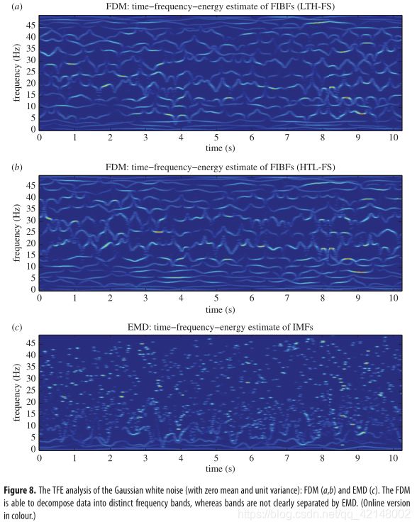
图8：高斯白噪声(均值和单位方差为零)的 的TFE分析:（a）（b）FDM，（c）EMD。FDM能够将数据分解成不同的频带，而EMD不能将频带清晰地分离出来。

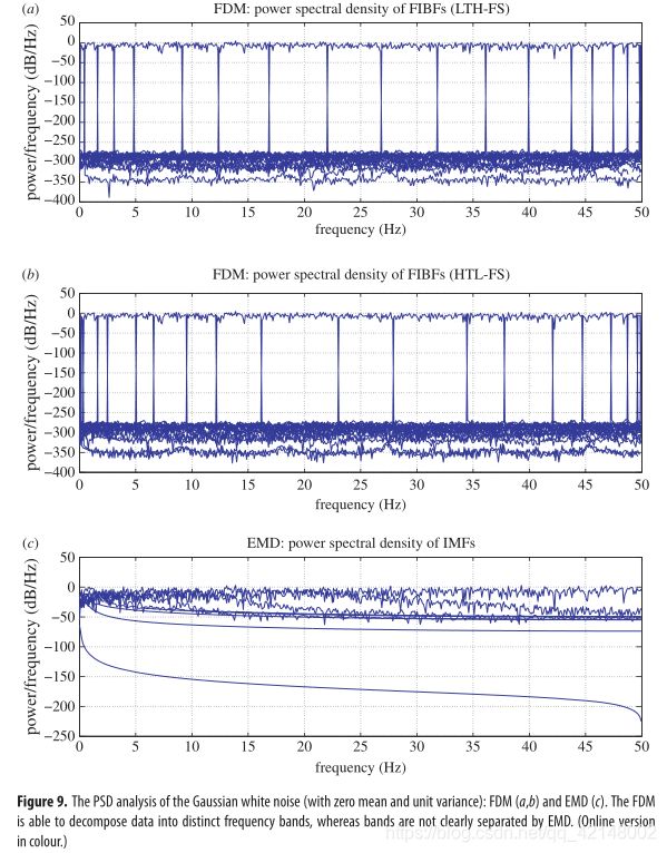
图9：高斯白噪声(均值和单位方差为零)的 的PSD分析:（a）（b）FDM，（c）EMD。FDM能够将数据分解成不同的频带，而EMD不能将频带清晰地分离出来。

(f) Time–frequency–energy analysis of unit sample sequence
(f) 单位样本序列的时间-频率-能量分析

The unit sample sequence is defined as $\delta [n-n_0]=1$ at $n=n_0$ and zero otherwise. By using the relation $z[n]=(1/\pi ){\int }_0^{\pi }X(\omega )\exp (j\omega n)d\omega$, we obtain the analytic representation of $x[n]=\delta [n-n_0]\iff X(\omega )=\exp (-j\omega n_0)$ as $$z[n]=\frac{\sin (\pi (n-n_0))+j[1-\cos (\pi (n-n_0))]}{\pi (n-n_0)}=a[n]\exp (j\varphi [n]),(5.4)$$
where the real part of $z[n]$ is $\delta [n-n_0]=\sin (\pi (n-n_0))/\pi (n-n_0),a[n]=|\sin ((\pi /2)(n-n_0))/(\pi /2)(n-n_0))|,\varphi [n]=(\pi /2)(n-n_0)$ and hence $\omega [n]=\pi /2$ which corresponds to half of the Nyquist frequency , that is $F_s$/4 Hz . Figure 10 shows the plots of the real part, imaginary part and absolute value of $z[n]$ with $n_0=199$, sampling frequency $F_s$=100 Hz, length $N$ =400. Theoretically , this clearly indicates that most of the energy of signal $\delta [n-n_0]$ is concentrated at time $t$=1.99 s ($n_0$=199) and frequency $f$ =25 Hz. Figure 11 shows the plots of FIBFs obtained by the FDM and figure 12 shows the TFE analysis of unit sample sequence $\delta [n-n_0]$ from the FDM , EEMD and continuous wavelet transform (CWT) methods. These figures clearly indicate that the TFE plot obtained by the FDM is the same as the theoretical estimation, whereas there is energy spread over a range of frequencies and lack of accuracy in the TFE plots obtained by the EEMD and CWT methods.

单位样本序列定义为在 $n=n_0$ 时， $\delta [n-n_0]=1$ ，否则等于0。通过使用关系式 $z[n]=(1/\pi ){\int }_0^{\pi }X(\omega )\exp (j\omega n)d\omega$，$x[n]=\delta [n-n_0]\iff X(\omega )=\exp (-j\omega n_0)$ ，我们得到了解析表达式为
$$z[n]=\frac{\sin (\pi (n-n_0))+j[1-\cos (\pi (n-n_0))]}{\pi (n-n_0)}=a[n]\exp (j\varphi [n]),(5.4)$$
其中 $z[n]$ 的实部为 $\delta [n-n_0]=\sin (\pi (n-n_0))/\pi (n-n_0)，a[n]=|\sin ((\pi /2)(n-n_0))/(\pi /2)(n-n_0))|，\varphi [n]=(\pi /2)(n-n_0)$，因此 $\omega [n]=\pi /2$ 对应于 Nyquist 采样频率的一半，即 $F_s$/4 Hz 。图10给出了 $z[n]$ 在 $n_0=199$，采样频率为 $F_s$=100 Hz，长度 $N$ =400 时的实部、虚部和绝对值的曲线图。理论上，这清楚地表明，信号 $\delta [n-n_0]$ 的大部分能量集中在时间 $t$=1.99 s ($n_0$=199) 频率 $f$ =25 Hz 上。 图11为FDM得到的FIBFs图，图12为FDM，EEMD和连续小波变换（CWT）方法对单元样本序列 $\delta [n-n_0]$ 分析图。这些数字清楚地表明，FDM得到的TFE图与理论估计相同，但能量在一个频率范围内分散，而EEMD和CWT方法得到的TFE图缺乏精确性。

图10. $\delta [n-n_0]$（$n_0=199$，采样频率为 $F_s$=100 Hz，长度 $N$ =400）的解析表达式：（a）$z[n]$ 的实部，（b）$z[n]$ 的虚部，（c）$z[n]$ 的绝对值。

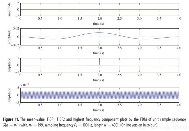
图11. 对单位采样序列 $\delta [n-n_0]$（$n_0=199$，采样频率为 $F_s$=100 Hz，长度 $N$ =400）进行FDM，得到均值、FIBF1、FIBF2和最高频率分量图。


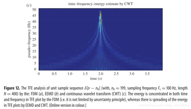
图12. 对单位采样序列 $\delta [n-n_0]$（$n_0=199$，采样频率为 $F_s$=100 Hz，长度 $N$ =400）的TFE分析：（a）FDM ，（b）EEMD，（c）连续小波变换(CWT)。FDM在TFE图中能量同时集中在时间和频率上(即不受不确定性原理的限制)，而EEMD和CWT在TFE图中能量在扩散。

The IF is defined through differentiation of phase rather than integration and hence overcomes the restriction of the uncertainty principle [34]. One can obtain arbitrary precision in time and frequency resolution subject only to the sampling rate in the case of discrete time signals. The uncertainty principle, in the context of signal analysis, states that the finer the time resolution one wants, the cruder would be the resulting frequency resolution. However, this example clearly demonstrates that the FHS obtained by FDM is indeed not limited by the uncertainty principle and a signal can be highly concentrated in both time and frequency domain, as shown in figure 12a.

通过对相位的微分而不是积分来定义IF，从而克服了不确定性原理[34]的限制。在离散时间信号的情况下，只受采样率的影响，可以获得任意精度的时间和频率分辨率。在信号分析的背景下，不确定性原理指出，想要的时间分辨率越精细，得到的频率分辨率就越粗糙。这个例子清楚地表明，由FDM获得的FHS确实不受不确定性原理的限制，并且信号可以在时域和频域中高度集中，如图12a所示。

Discussion: It is to be noted that the FHS provides time and average frequency distribution. In order to explain the average frequency effects, we consider a sum of sinusoids of equal amplitudes $x(t)={\sum }_{k=1}^{N}A\cos ({\omega }_{0}kt)$. Its analytic representation is given by $z(t)={\sum }_{k=1}^{N}A\exp (j{\omega }_{0}kt)=(A\sin ({\omega }_0(N/2)t)/\sin ({\omega }_{0}t/2))\exp (j{\omega }_0((N+1)/2)t)=a(t)\exp (j\varphi (t))$, which implies phase $\varphi (t)=({\omega }_0((N+1)/2)t)$ and hence IF $f(t)=(1/2\pi ){\omega }_0((N+1)/2)$. This is what we observe in these figures (especially figure 12a). It is also to be noted that if amplitudes of the constituent sinusoids are not equal, then the resultant IF would not be a constant (average) frequency , that is it would be a time-varying frequency .

讨论： 值得注意的是，FHS提供了时间和平均频率分布。为了解释平均频率效应，我们考虑幅度相等的正弦曲线之和 $x(t)={\sum }_{k=1}^{N}A\cos ({\omega }_{0}kt)$。他的解析表达式为 $z(t)={\sum }_{k=1}^{N}A\exp (j{\omega }_{0}kt)=(A\sin ({\omega }_0(N/2)t)/\sin ({\omega }_{0}t/2))\exp (j{\omega }_0((N+1)/2)t)=a(t)\exp (j\varphi (t))$，这意味着其相位为 $\varphi (t)=({\omega }_0((N+1)/2)t)$，因此 IF为 $f(t)=(1/2\pi ){\omega }_0((N+1)/2)$。这就是我们在这些图中观察到的(尤其是图12a)。还需要注意的是，如果组成正弦波的振幅不相等，那么合成的 IF 将不是一个常数(平均)频率，也就是说，它将是一个时变频率

(g) Application to earthquake data analysis
(g) 地震数据分析应用

Earthquake time series signals are nonlinear and non-stationary in character. The El Centro earthquake data (sampled at $F_s$=50 Hz) has been taken from (http://www.vibrationdata.com/elcentro.htm) and is shown in figure 13. The critical frequency range that matters in the structural design is less than 10 Hz, and from the Fourier-based PSD, marginal spectrum by FDM and marginal spectrum by EMD, one can observe that almost all the energy in this data, as shown in figure 13, lies within 10 Hz. The IE fluctuations of the El Centro earthquake data estimated by the FDM and EMD methods are shown in figure 14. The IE estimated by the EMD has some transient and rapid fluctuations, whereas the IE estimated by the FDM appears smoother than the EMD case. The TFE distribution by the FDM, EMD and CWT methods are shown in figure 15, and all three methods indicate maximum energy concentration around 1.7 Hz and 2 s. There is enhanced TFE tracking by the FDM as it provides better and finer details of how the different waves arrive from the epical centre to the recording station, for example the compression waves of small amplitude but higher frequency range of 10–20Hz, the shear and surface waves of strongest amplitude and lower frequency range of below 5Hz which does most of the damage, and other body shear waves which are present over the full duration of the data span.

地震时间序列信号具有非线性、非平稳的特点。El Centro地震数据($F_s$=50 Hz 采样)取自(http://www.vibrationdata.com/elcento .htm)，如图13所示。结构设计中重要的临界频率范围小于10 Hz，从基于傅立叶的PSD、FDM的边际谱和EMD的边际谱可以看出，该数据中几乎所有的能量都在10 Hz 以内，如图13所示。FDM和EMD方法估计的El Centro地震数据的IE波动如图14所示。由EMD估计的IE有一些瞬态和快速的波动，而由FDM估计的IE比EMD估计的看起来更平滑。FDM、EMD和CWT方法的TFE分布如图15所示，这三种方法都表明最大能量集中在1.7 Hz 和 2 s 左右。FDM增强了TFE跟踪，因为它提供了不同波如何从中心传播到记录站的更好和更精细的细节，例如振幅小但频率范围较高(10–20 Hz)的压缩波、振幅最强且频率范围较低(5 Hz 以下)的剪切波和表面波，它们造成了大部分损害，以及在整个数据跨度期间存在的其他体剪切波。


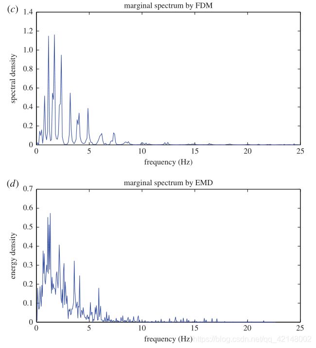
图13.（a）1940年5月18日 El Centro地震的南北分量图，（b）基于傅立叶的功率谱密度(PSD)，（c）FDM的边际谱，（d） EMD的边际谱。

图14. El Centro地震资料的瞬时能量密度 $E(t)$ 图：（a）FDM（b）EMD。


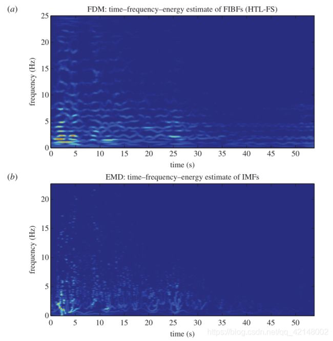
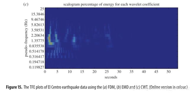
图15. El Centro地震资料的TFE图：（a）FDM，（b）EMD，（c）CWT。

(h) Application to speech signal analysis
(h) 语音信号分析应用

Finally , to illustrate the advantages of FDM in speech signal analysis, we decompose a quasiperiodic voice signal (long vowel ‘I’). In figure 16, the FIBFs $y_2–y_5$ seem to extract most of the noise, while $y_6$ to $y_7$ seem to express most of the signal information at high frequencies. Moreover, the FIBF $y_8$ captures accurately $F_0$, the fundamental frequency (inverse of glottal pulse or pitch period length) of the voice signal. By contrast, the EMD (figure 17a) presents mode mixing between modes 2 and 3, between modes 3 and 4 and between modes 4 and 5. Also, the EMD is not able to capture $F_0$ in any mode. In figure 17b, the EEMD is able to capture $F_0$ in mode $y_5$, although it can be observed that appearance of positive minima and negative maxima in the mode $y_4$ and $y_7$, which is a violation of the first IMF condition. The EEMD modes $y_3$ and $y_4$ are a asymmetric waveform which is a violation of the second IMF condition. Besides these problems, the major drawbacks in this case are huge computation complexity for this ensemble size and the reconstruction error that may be significant. The computation complexity can be reduced by selecting the smaller ensemble size but that increases the reconstruction error. Figure 18 shows the plots of TFE distribution obtained by the FDM, EMD and EEMD algorithms for same data (long vowel ‘I’). Clearly , there is enhanced TFE tracking when using the FDM. The results in this application as well are in clear favour of the Fourier method proposed in this paper.

最后，为了说明FDM在语音信号分析中的优势，我们分解了一个准周期语音信号(长元音‘I’)。在图16中，FIBFs $y_2–y_5$ 似乎提取了大部分噪声，而 $y_6$ 至 $y_7$ 似乎表达了高频下的大部分信号信息。另外，FIBF $y_8$ 能够准确捕捉语音信号的基频 $F_0$ (声门脉冲或基音周期长度的倒数)。相比之下，EMD (图17a) 呈现了模式2和模式3之间、模式3和模式4之间以及模式4和模式5之间的模式混合。此外，EMD在任何模式下都无法捕获 $F_0$ 。在图17b中，EEMD 可以在模式 $y_5$ 中捕获 $F_0$ ，但可以观察到在 $y_4$ 和 $y_7$ 模式中出现了正极小值和负极大值，这违反了第一IMF条件。EEMD模态 $y_3$ 和$y_4$ 是非对称波形，违反了第二个IMF条件。除了这些问题之外，这种情况下的主要缺点是对于这种集合大小的巨大计算复杂性和可能显著的重建误差。选择较小的集成规模可以降低计算复杂度，但会增加重构误差。图18给出了相同数据(长元音’ I ‘)采用FDM、EMD和EEMD算法得到的TFE分布曲线图。显然，在使用FDM时增强了TFE跟踪。应用结果也明显支持本文提出的傅里叶方法。

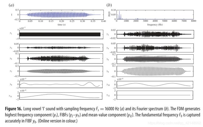
图16. 长元音’ I '音，采样频率$F_s$=16000 Hz，（a）傅里叶频谱，（b）FDM产生最高频率分量($y_1$)、FIBFs分量($y_2-y_{11}$)和均值分量($y_{12}$)。FIBFs $y_8$ 能准确捕捉基频 $F_0$。

6. Conclusion
6.结论

In this paper, we have proposed (i) a novel and adaptive FDM for nonlinear and non-stationary time series analysis, which decomposes any data into a small number of band-limited FIBFs. The FDM is a generalized Fourier expansion with variable amplitudes and variable frequencies of a time series by the Fourier method itself. (ii) The zero-phase filter bank-based MFDM algorithm, for the analysis of multivariate nonlinear and non-stationary time series, which generates a finite number of band limited multivariate FIBFs (MFIBFs). (iii) An algorithm to obtain cut-off frequencies required in MFDM for zero-phase high or low pass filtering of multivariate signals.

在本文中，我们提出了

(i)一种用于非线性和非平稳时间序列分析的新型自适应FDM，它将任何数据分解成少量的带限FIBFs。FDM是傅里叶方法本身对时间序列的变幅变频率的广义傅里叶展开。

(ii)基于零相位滤波器组的MFDM算法，用于分析多元非线性和非平稳时间序列，生成有限个带限多元 FIBFs (MFIBFs)。

(iii)对多元信号进行零相位高低通滤波时，获得MFDM所需截止频率的算法。

The fundamental and conceptual contributions of this study are the Fourier based adaptive signal decomposition method (FDM) and the introduction of the FIBFs. The FIBFs form the basis of the decomposition that are complete, orthogonal, local and adaptive. The instantaneous frequencies of the FIBFs yield TFE distribution of any signal. The TFE distribution of a signal is used in various fields of science and engineering for analysis of physical phenomena and engineering systems. The proposed methods produce the final presentation of the results as a TFE distribution that reveals the imbedded structures of a signal. Unlike the various EMD algorithms, the FDM and MFDM are mathematically well defined, supported by the well-established theories of a zero-phase filter and the FTs. The FDM and MFDM do not suffer from the limitations with regard to mode mixing, detrend uncertainty and end effect artefacts of EMD algorithms. Simulation results clearly demonstrate the efficacy of the proposed methods.

本研究的基础和概念贡献是基于傅立叶的自适应信号分解方法(FDM)和FIBFs的引入。FIBFs构成了完全、正交、局部和自适应分解的基础。FIBFs的瞬时频率产生任何信号的TFE分布。信号的TFE分布在科学和工程的各个领域中用于物理现象和工程系统的分析。所提出的方法产生结果的最终表示为TFE分布，该分布揭示了信号的嵌入结构。与各种EMD算法不同的是，FDM和MFDM在数学上有很好的定义，并得到了完善的零相位滤波器和FTs理论的支持。FDM和MFDM不受EMD算法的模态混合、去趋势不确定性和端点效应的限制。仿真结果清楚地证明了该方法的有效性。