吴恩达ML WEEK3 练习一代码(线性回归)
吴恩达机器学习 第三周
- 0 总结
- 1 简单MATLAB函数
-
- 1.2 warmUpExercise.m
- 2 单变量线性回归
- 2.1 绘制
-
- 2.2 梯度下降
-
- 2.2.1 更新公式
- 2.2.2 实施
- 2.2.3 完成代价函数的计算
- 2.2.4 梯度下降
- 3 多变量线性回归
-
- 3.1 特征归一化
- 3.2 梯度下降
-
- 3.2.1 预测
- 3.3 正规方程
0 总结
学习时间:2022.9.12~2022.9.18
- 复习单变量线性回归和多变量线性回归
- 复习MATLAB软件的使用
- 利用所学知识,完成单变量线性回归代价函数计算、梯度下降的代码编写
- 利用所学知识,完成多变量线性回归代价函数计算、梯度下降的代码编写,以及正规方程法求解 θ \theta θ的代码编写。
- 熟悉了使用梯度下降法求解线性回归的流程和代码,可以很好地运用MATLAB求解问题
1 简单MATLAB函数
1.2 warmUpExercise.m
用途:返回5*5的单位阵。
代码:
function A = warmUpExercise()
	A = eye(5);
end
2 单变量线性回归
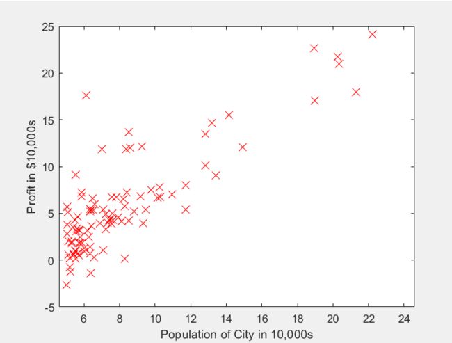
问题描述:ex1data1.txt包含所有数据集,第一列是城市的人口,第二列是该城市的收益(负数表示亏本)。你需要使用这个数据预测下一个扩张的城市。
2.1 绘制
任务:补充plotData.m,绘制数据。
代码:
function plotData(x, y)
	figure; % open a new figure window
	plot(x,y,'rx','MarkerSize',10);
	ylabel('Profit in $10,000s');
	xlabel('Population of City in 10,000s');
end
运行结果:
2.2 梯度下降
任务:计算线性回归参数 θ \theta θ。
2.2.1 更新公式
假设函数是关于 x x x的函数: h θ ( x ) = θ T x = θ 0 + θ 1 x h_\theta(x)=\theta^Tx=\theta_0+\theta_1x hθ(x)=θTx=θ0+θ1x代价函数是关于 θ 0 , θ 1 \theta_0,\theta_1 θ0,θ1的函数:
J ( θ ) = 1 2 m ∑ i = 1 m ( h θ ( x i ) − y i ) 2 J(\theta)=\frac{1}{2m}\sum^{m}_{i=1}(h_\theta(x^{i})-y^{i})^{2} J(θ)=2m1i=1∑m(hθ(xi)−yi)2优化目标是寻求使得代价函数最小的 θ 0 , θ 1 \theta_0,\theta_1 θ0,θ1: min θ 0 , θ 1 J ( θ ) \min_{\theta_0,\theta_1}J(\theta) θ0,θ1minJ(θ)其中一个方法是使用梯度下降,每次迭代过程中的更新公式:

2.2.2 实施
在此前,我们已经导入了数据,x和y都是m列的数据,其中x中每一行表示每一个样本,为了与 θ \theta θ相匹配,我们需要给x每一行增加一个 x 0 x_0 x0=1。初始化迭代次数为1500,学习率为0.01。
代码:
X = [ones(m, 1), data(:,1)]; % Add a column of ones to x
theta = zeros(2, 1); % initialize fitting parameters

% Some gradient descent settings
iterations = 1500;
alpha = 0.01;
2.2.3 完成代价函数的计算
任务:完成computeCost.m
代码:
function J = computeCost(X, y, theta)
%COMPUTECOST Compute cost for linear regression
%   J = COMPUTECOST(X, y, theta) computes the cost of using theta as the
%   parameter for linear regression to fit the data points in X and y

% Initialize some useful values
m = length(y); % number of training examples

% You need to return the following variables correctly
J = 0;

% ====================== YOUR CODE HERE ======================
% Instructions: Compute the cost of a particular choice of theta
%               You should set J to the cost.
h = X*theta; % m*1的矩阵,每一行对应每个样本的预测值h
J = 1/(2*m)*sum((h-y).^2);
% =========================================================================

end
运行结果:

2.2.4 梯度下降
任务:完成gradientDescent.m
代码:
function [theta, J_history] = gradientDescent(X, y, theta, alpha, num_iters)
%GRADIENTDESCENT Performs gradient descent to learn theta
%   theta = GRADIENTDESCENT(X, y, theta, alpha, num_iters) updates theta by
%   taking num_iters gradient steps with learning rate alpha

% Initialize some useful values
m = length(y); % number of training examples
J_history = zeros(num_iters, 1); % 记录每次迭代得到的J,如果正确的话是按迭代次数递减的

for iter = 1:num_iters

    % ====================== YOUR CODE HERE ======================
    % Instructions: Perform a single gradient step on the parameter vector
    %               theta.
    %
    % Hint: While debugging, it can be useful to print out the values
    %       of the cost function (computeCost) and gradient here.
    %
    h = X*theta; % m*1的矩阵,每一行对应每个样本的预测值h
    theta = theta - alpha / m * (X' * (h - y));
    % ============================================================

    % Save the cost J in every iteration
    J_history(iter) = computeCost(X, y, theta);

end

end
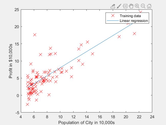
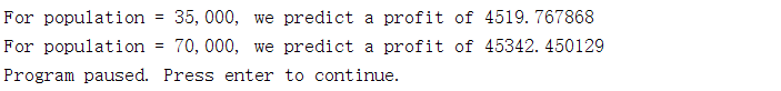
结果:

3 多变量线性回归
问题描述:ex1data2.txt包含了关于房价的所有数据集,第一列是房子大小,第二列是卧室数量,第三列是房子价格。
3.1 特征归一化
x n ( i ) = x n ( i ) − u n s n x_n^{(i)}=\frac{x_n^{(i)}-u_n}{s_n} xn(i)=snxn(i)−un其中, u n u_n un是平均值, s n s_n sn是标准差,也可以用最大值-最小值代替。这样算得的x会在-0.5到0.5之间。
任务:完成featureNormalize.m中的代码,首先计算平均值存在mu数组,然后除以标准差(standard deviation)
代码:
function [X_norm, mu, sigma] = featureNormalize(X)
%FEATURENORMALIZE Normalizes the features in X
%   FEATURENORMALIZE(X) returns a normalized version of X where
%   the mean value of each feature is 0 and the standard deviation
%   is 1. This is often a good preprocessing step to do when
%   working with learning algorithms.

% You need to set these values correctly
X_norm = X;
mu = zeros(1, size(X, 2)); % size(X, 2)特征数
sigma = zeros(1, size(X, 2));

% ====================== YOUR CODE HERE ======================
% Instructions: First, for each feature dimension, compute the mean
%               of the feature and subtract it from the dataset,
%               storing the mean value in mu. Next, compute the
%               standard deviation of each feature and divide
%               each feature by it's standard deviation, storing
%               the standard deviation in sigma.
%
%               Note that X is a matrix where each column is a
%               feature and each row is an example. You need
%               to perform the normalization separately for
%               each feature.
%
% Hint: You might find the 'mean' and 'std' functions useful.
% 平均值储存在mu,标准差储存在sigma
mu = mean(X,1); % 计算每一列的均值,1表示列
sigma = std(X,1); 5 计算每一行的标准差,1表示列
% X = (X-mu)./sigma;
for i=1:size(X,2)
    % 对每一列X做如下操作
    % 易错点:起初把i写成了1
    X_norm(:,i) = (X(:,i)-mu(i))./sigma(i);
end
% ============================================================

end
3.2 梯度下降
任务:完成多特征回归的梯度下降,完成computeCostMulti.m 和gradientDescentMulti.m的代码。
提示:可以用size(X,2)看有多少特征。
computeCostMulti.m代码(和单变量一样):
function J = computeCostMulti(X, y, theta)
%COMPUTECOSTMULTI Compute cost for linear regression with multiple variables
%   J = COMPUTECOSTMULTI(X, y, theta) computes the cost of using theta as the
%   parameter for linear regression to fit the data points in X and y

% Initialize some useful values
m = length(y); % number of training examples

% You need to return the following variables correctly
J = 0;

% ====================== YOUR CODE HERE ======================
% Instructions: Compute the cost of a particular choice of theta
%               You should set J to the cost.
h = X * theta;
J = 1/(2*m)*sum((h-y).^2);
% =========================================================================

end
gradientDescentMulti.m代码(和单变量一样):
function [theta, J_history] = gradientDescentMulti(X, y, theta, alpha, num_iters)
%GRADIENTDESCENTMULTI Performs gradient descent to learn theta
%   theta = GRADIENTDESCENTMULTI(x, y, theta, alpha, num_iters) updates theta by
%   taking num_iters gradient steps with learning rate alpha

% Initialize some useful values
m = length(y); % number of training examples
J_history = zeros(num_iters, 1);

for iter = 1:num_iters

    % ====================== YOUR CODE HERE ======================
    % Instructions: Perform a single gradient step on the parameter vector
    %               theta.
    %
    % Hint: While debugging, it can be useful to print out the values
    %       of the cost function (computeCostMulti) and gradient here.
    %
    h = X * theta;
    theta = theta - alpha / m * (X' * (h - y));
    % ============================================================

    % Save the cost J in every iteration
    J_history(iter) = computeCostMulti(X, y, theta);

end

end
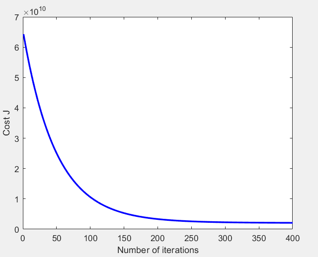
运行结果:
①随着每次迭代代价函数的变化:
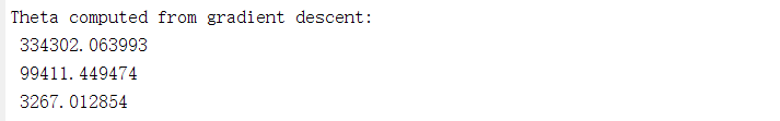
②得到的 θ \theta θ值:
3.2.1 预测
预测面积为1650,卧室个数为3的房子价格
预测结果是$289221.547371
% Estimate the price of a 1650 sq-ft, 3 br house
% ====================== YOUR CODE HERE ======================
% Recall that the first column of X is all-ones. Thus, it does
% not need to be normalized.
X_test = [1650 3];
X_test = [1 (X_test-mu)./sigma];
y_predict = X_test*theta;
3.3 正规方程
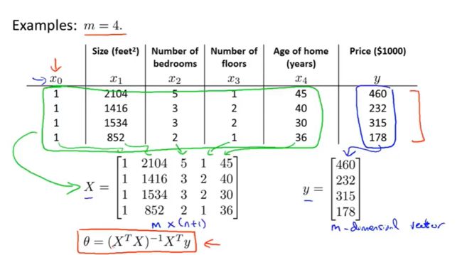
任务:完成normalEqn.m,实现正规方程对 θ \theta θ的求解。
只需在normalEqn.m中加入一行代码:
theta = pinv(X'*X)*X'*y;
运行结果:

 —
—