如何使用双线性变换法将模拟电路滤波器设计成为数字滤波器？

信号处理（数字模拟信号）

1.1 双线性变换设计递归滤波器

• 设计滤波器¹

1. 试着写出双线性变换法设计IIR数字高通滤波器的主要步骤
   • 将数字高通的频率指标转换为模拟高通的频率指标（其中将高通截止频率通过预畸转换为模拟高通的截止频率）
   • 将模拟高通技术指标转换成为模拟低通技术指标
   • 设计模拟低通原型滤波器
   • 将模拟低通原型滤波器通过双线形映射为数字低通原型滤波器（下面一小节主要介绍这方面的工作）

（理解主要就是，将频率滤波的带宽从数字转换到模拟信号，再将相应的技术指标从模拟高通到模拟低通，然后设计一个相应的低通的模拟滤波器，再使用双线性映射到数字低通滤波器）

2. 简述用窗函数法设计FIR滤波器的时，对理想低通滤波器加矩形窗处理后的影响；为了改善FIR的性能，窗函数要尽可能的满足什么样的条件？
   • 幅频特性的陡直边沿被加宽，形成一个过渡带，其带宽取决于窗函数频响的主瓣宽度
   • 过渡带的两侧附近产生起伏的尖峰和波纹，这是由于窗函数旁瓣引起的
   • 增加截取长度N，将缩小窗函数主瓣宽度，但不能减小旁瓣的宽度值；能减小过渡带的宽度；能减小过渡带宽度，但不能改善带通内的平稳性和阻带衰减
   • 为改善滤波器性能，窗函数需要满足：
     （1）主瓣宽度尽量窄，以获得较陡的过渡带
     （2）旁瓣值尽可能的小，以改善通带的平稳度和增大阻带的衰减。

1.2 相关数学内容

这里²详细介绍了矩形函数、三角函数与高斯函数的傅立叶变换的推导过程。

1.3 matlab设计

0）设计过程

• Matlab实现IIR数字滤波器设计
• 傅立叶变换、拉普拉斯变换、Z变换之间的联系？
• 滤波器的各个段的表示

1）画出滤波器频谱

设计工具：画出幅度谱与频谱图

N = 512;
H = fft(b,N)./fft(a,N);   % H矩阵
mag = 20*log10(abs(H));    % get magnitude of spectrum in dB 幅值
phase = angle(H)*2*pi;     % get phase in deg.相位
faxis = fs/2*linspace(0,1,N/2);  % the axis of frequency

figure,
subplot(2,1,1),plot(faxis,mag(1:N/2))
xlabel('Frequency (Hz)'),ylabel('Magnitude (dB)')
grid on
subplot(2,1,2),plot(faxis,phase(1:N/2),'r')
xlabel('Frequency (Hz)'),ylabel('Phase (deg.)')
grid on
figure;freqz(b,a)	%%这个画出来的信号坐标轴应该乘一个fs采样率

结果如下，可见两者基本一致。（带通椭圆数字滤波器 ）

2）利用函数设计滤波器

Rp =3; Rs =30 ;%%设计一个带通椭圆数字滤波器 , 通带为 100 ～200 H z,过渡带均为 50 H z,
% 通带波纹小于 3 db ,阻带衰减为 30 db 
Wp =2 *[ 100 200] /fs;
Ws = 2 *[ 80 220] /fs;
[ n , Wn] = ellipord (Wp , Ws , Rp , Rs);
[ b , a] = ellip(n , Rp, Rs,Wn);
dataOut = filter(b,a,yc);
figure;NN = length(yc);plot((-NN/2+1:NN/2)/NN*fs,20*log10(abs(fftshift(fft(yc)))),'LineWidth',2);axis([-inf,inf,-inf,inf]);xlabel('fs Hz');ylabel('幅度谱 dB');hold on;
N = length(dataOut);x = (-N/2+1:N/2)/N*fs;semilogy(x , abs(fftshift(fft(dataOut))) ,'r');legend 采样后 滤波后

3）给滤波器进行加窗

一、FIR滤波器
加窗过程是对FIR滤波器系数b矩阵进行计算：

w = kaiser(N,beta);
h = b.*w';% 设计的滤波器
mag = freqz(h,[1],omega);

b矩阵相当于“系统的单位冲激响应（时域上）”，而利用freqz函数可以转换到频域上观察幅度谱与相位谱，可以清晰看到滤波器的抖动有所改善。

下面讨论了为什么可以对滤波器系数a、b矩阵进行fft处理。freqz函数的作用是将传递函数/z函数转换成为频域的单位冲激响应。以及为什么需要对h(t)进行加窗。

因此，FIR的系数常常以sinc函数的形式呈现，其傅立叶变换之后在频域上的信号便为类似一个矩阵的形状。
二、IIR滤波器
认为IIR滤波器会有不一样的表现形式。因为其系数是在分母的位置。

H = fft(b,N)./fft(a,N);

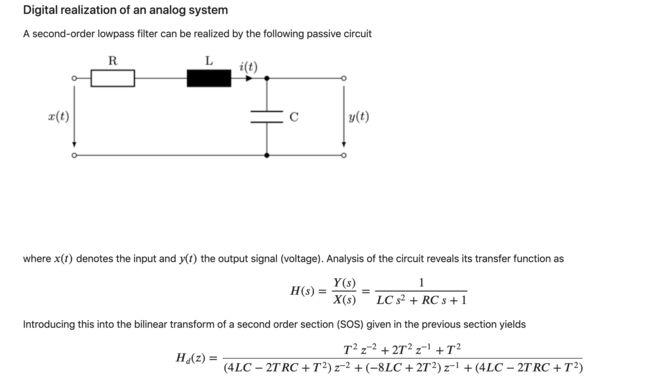
2 模拟电路滤波器到数字滤波器（双线性变换设计滤波器）

2.1 原理部分³

做如下运算笔记内容：

2.1.2 选取示例

下面展示了python代码：

import scipy.signal as sig


fs = 44100  # sampling frequency
fc = 1000  # corner frequency of the lowpass

# coefficients of analog lowpass filter 模拟低通滤波器系数
Qinf = 0.8
sinf = 2*np.pi*fc 
C = 1e-6
L = 1/(sinf**2*C)
R = sinf*L/Qinf

B = [0, 0, 1]
A = [L*C, R*C, 1]

# cofficients of digital filter
T = 1/fs
b = [T**2, 2*T**2, T**2]
a = [(4*L*C+2*T*R*C+T**2), (-8*L*C+2*T**2), (4*L*C-2*T*R*C+T**2)]

fs2 = 64100
T2 = 1/fs2
b2 = [T2**2, 2*T2**2, T2**2]
a2 = [(4*L*C+2*T2*R*C+T2**2), (-8*L*C+2*T2**2), (4*L*C-2*T2*R*C+T2**2)]

# compute frequency responses
Om, Hd = sig.freqz(b, a, worN=1024)#离散的
Om2, Hd2 = sig.freqz(b2, a2, worN=1024)#离散的
tmp, H = sig.freqs(B, A, worN=fs*Om)# 连续的模拟信号

# plot results
f = Om*fs/(2*np.pi)
plt.figure(figsize=(10, 4))
plt.semilogx(f, 20*np.log10(np.abs(H)),
             label=r'$|H(j \omega)|$ of analog filter')
plt.semilogx(f, 20*np.log10(np.abs(Hd)),
             label=r'$|H_d(e^{j \Omega})|$ of digital filter fs = 44100')
plt.semilogx(f, 20*np.log10(np.abs(Hd2)),
             label=r'$|H_d(e^{j \Omega})|$ of digital filter fs = 64100')
plt.xlabel(r'$f$ in Hz')
plt.ylabel(r'dB')
plt.axis([100, fs/2, -70, 3])
plt.legend()
plt.grid()

可以看到模拟电路的滤波器与数字电路的滤波器有如下的对应关系。此外，当采样频率越高（如下采样率为64100Hz时），其滤波器与模拟电路滤波器越接近。

---

1. 博客 - 数据处理与滤波器性质 ↩︎

2. https://blog.csdn.net/qq_22943397/article/details/80301398 ↩︎

3. 参考开源项目digital-signal-processing-lecture-master ↩︎