18_Reinforcement Learning_CartPole_reduce_mean_Q-Value Iteration_Q-learning_DQN_get_weights_replay

     Reinforcement Learning (RL) is one of the most exciting fields of Machine Learning today, and also one of the oldest. It has been around since the 1950s, producing many interesting applications over the years,(For more details, be sure to check out Richard Sutton and Andrew Barto’s book on RL, Reinforcement Learning: An Introduction (MIT Press).) particularly in games (e.g., TD-Gammon, a Backgammon-playing program) and in machine control, but seldom making the headline news. But a revolution took place in 2013, when researchers from a British startup called DeepMind demonstrated a system that could learn to play just about any Atari game from scratch,(Volodymyr Mnih et al., “Playing Atari with Deep Reinforcement Learning,” arXiv preprint arXiv:1312.5602 (2013).) eventually outperforming humans(Volodymyr Mnih et al., “Human-Level Control Through Deep Reinforcement Learning,” Nature 518 (2015): 529–533) in most of them, using only raw pixels as inputs and without any prior knowledge of the rules of the games.(Check out the videos of DeepMind’s system learning to play Space Invaders, Breakout, and other video games at https://homl.info/dqn3 OR https://www.youtube.com/watch?v=ePv0Fs9cGgU&list=PLkqhIF5RuX2c5SeAQE0wRw5gdOSjpixXI ) This was the first of a series of amazing feats, culminating[ˈkʌlmɪneɪtɪŋ]达到顶点 in March 2016 with the victory of their system AlphaGo against Lee Sedol, a legendary professional player of the game of Go, and in May 2017 against Ke Jie, the world champion. No program had ever come close to beating a master of this game, let alone the world champion. Today the whole field of RL is boiling with new ideas, with a wide range of applications. DeepMind was bought by Google for over $500 million in 2014.

     So how did DeepMind achieve all this? With hindsight it seems rather simple: they applied the power of Deep Learning to the field of Reinforcement Learning, and it worked beyond their wildest dreams. In this chapter we will first explain what Reinforcement Learning is and what it’s good at, then present two of the most important techniques in Deep Reinforcement Learning: policy gradients and deep Qnetworks (DQNs), including a discussion of Markov decision processes (MDPs). We will use these techniques to train models to balance a pole[poʊl]杆 on a moving cart; then I’ll introduce the TF-Agents library, which uses state-of-the-art algorithms that greatly simplify building powerful RL systems, and we will use the library to train an agent to play Breakout, the famous Atari game. I’ll close the chapter by taking a look at some of the latest advances in the field.

Learning to Optimize Rewards

     In Reinforcement Learning, a software agent makes observations and takes actions within an environment, and in return it receives rewards. Its objective is to learn to act in a way that will maximize its expected rewards over time. If you don’t mind a bit of anthropomorphism[ˌænθrəpəˈmɔːrfɪzəm]神人同形同性论, you can think of positive rewards as pleasure, and negative rewards as pain (the term “reward” is a bit misleading in this case). In short, the agent acts in the environment and learns by trial and error to maximize its pleasure and minimize its pain.

This is quite a broad setting, which can apply to a wide variety of tasks. Here are a few examples (see Figure 18-1):

• a. The agent can be the program controlling a robot. In this case, the environment is the real world, the agent observes the environment through a set of sensors such as cameras and touch sensors, and its actions consist of sending signals to activate motors. It may be programmed to get positive rewards whenever it approaches the target destination, and negative rewards whenever it wastes time or goes in the wrong direction.
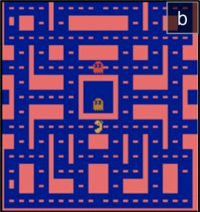
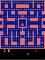
• b. The agent can be the program controlling Ms. Pac-Man. In this case, the environment is a simulation of the Atari game, the actions are the nine possible joystick positions (upper left, down, center, and so on), the observations are screenshots, and the rewards are just the game points.
• c. Similarly, the agent can be the program playing a board game such as Go.
• d. The agent does not have to control a physically (or virtually) moving thing. For example, it can be a smart thermostat[ˈθɜːrməstæt]自动调温器 , getting positive rewards whenever it is close to the target temperature and saves energy, and negative rewards when humans need to tweak the temperature, so the agent must learn to anticipate[ænˈtɪsɪpeɪt] 预计（并做准备） human needs.
• e. The agent can observe stock market prices and decide how much to buy or sell every second. Rewards are obviously the monetary[ˈmɑːnɪteri]货币的  gains and losses.

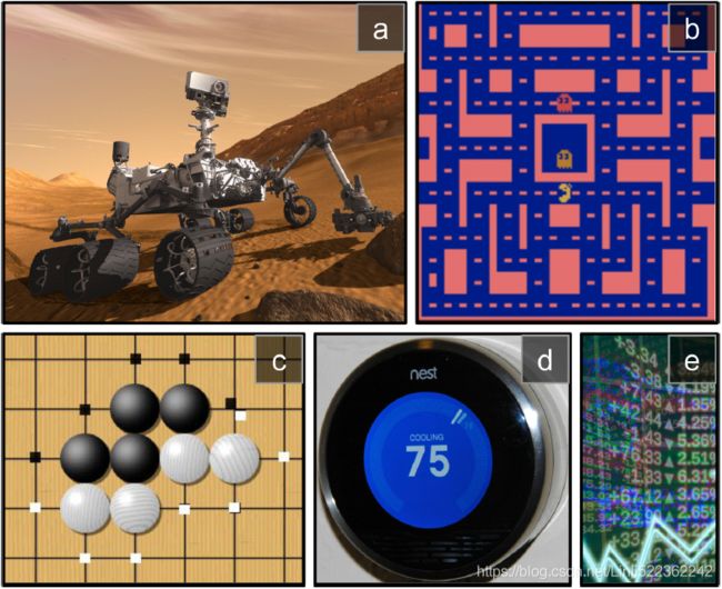Figure 18-1. Reinforcement Learning examples: (a) robotics, (b) Ms. Pac-Man, (c) Go player, (d) thermostat, (e) automatic trader (Image (a) is from NASA (public domain). (b) is a screenshot from the Ms. Pac-Man game, copyright Atari (fair use in this chapter). Images (c) and (d) are reproduced from Wikipedia. (c) was created by user Stevertigo and released under Creative Commons BY-SA 2.0. (d) is in the public domain. (e) was reproduced from Pixabay, released under Creative Commons CC0.) 

     Note that there may not be any positive rewards at all; for example, the agent may move around in a maze[meɪz]迷宫,使混乱, getting a negative reward at every time step, so it had better find the exit as quickly as possible! There are many other examples of tasks to which Reinforcement Learning is well suited, such as self-driving cars, recommender systems, placing ads on a web page, or controlling where an image classification system should focus its attention.

Policy Search

     The algorithm a software agent uses to determine its actions is called its policy策略. The policy could be a neural network taking observations as inputs and outputting the action to take (see Figure 18-2).
Figure 18-2. Reinforcement Learning using a neural network policy

     The policy can be any algorithm you can think of, and it does not have to be deterministic[dɪˌtɜːrmɪˈnɪstɪk]确定性的. In fact, in some cases it does not even have to observe the environment! For example, consider a robotic vacuum cleaner whose reward is the amount of dust it picks up in 30 minutes. Its policy could be to move forward with some probability p every second, or randomly rotate left or right with probability 1 – p. The rotation angle would be a random angle between –r and +r. Since this policy involves some randomness, it is called a stochastic policy. The robot will have an erratic trajectory[trəˈdʒektəri] [物] 轨道，轨线, which guarantees that it will eventually get to any place it can reach and pick up all the dust. The question is, how much dust will it pick up in 30 minutes?

     How would you train such a robot? There are just two policy parameters you can tweak: the probability p and the angle range r. One possible learning algorithm could be to try out many different values for these parameters, and pick the combination that performs best (see Figure 18-3). This is an example of policy search, in this case using a brute [bruːt] force approach蛮力方法. When the policy space is too large (which is generally the case), finding a good set of parameters this way is like searching for a needle in a gigantic[dʒaɪˈɡæntɪk]巨大的 haystack[ˈheɪstæk]干草堆.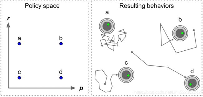
Figure 18-3. Four points in policy space (left) and the agent’s corresponding behavior (right)

     Another way to explore the policy space is to use genetic algorithms. For example, you could randomly create a first generation of 100 policies and try them out, then “kill” the 80 worst policies (It is often better to give the poor performers a slight chance of survival, to preserve some diversity in the “gene pool.”) and make the 20 survivors produce 4 offspring each. An offspring is a copy of its parent (If there is a single parent, this is called asexual[ˌeɪˈsekʃuəl]无性生殖的  reproduction. With two (or more) parents, it is called sexual reproduction. An offspring’s genome (in this case a set of policy parameters) is randomly composed of parts of its parents’ genomes) plus some random variation. The surviving policies plus their offspring together constitute the second generation. You can continue to iterate through generations this way until you find a good policy.

     Yet another approach is to use optimization techniques, by evaluating the gradients of the rewards with regard to the policy parameters, then tweaking these parameters by following the gradients toward higher rewards.(This is called Gradient Ascent. It’s just like Gradient Descent but in the opposite direction: maximizing instead of minimizing.) We will discuss this approach, is called policy gradients (PG), in more detail later in this chapter. Going back to the vacuum cleaner robot, you could slightly increase p and evaluate whether doing so increases the amount of dust picked up by the robot in 30 minutes; if it does, then increase p some more, or else reduce p. We will implement a popular PG algorithm using TensorFlow, but before we do, we need to create an environment for the agent to live in—so it’s time to introduce OpenAI Gym.

Introduction to OpenAI Gym

     One of the challenges of Reinforcement Learning is that in order to train an agent, you first need to have a working environment. If you want to program an agent that will learn to play an Atari game, you will need an Atari game simulator. If you want to program a walking robot, then the environment is the real world, and you can directly train your robot in that environment, but this has its limits: if the robot falls off a cliff, you can’t just click Undo. You can’t speed up time either; adding more computing power won’t make the robot move any faster. And it’s generally too expensive to train 1,000 robots in parallel. In short, training is hard and slow in the real world, so you generally need a simulated environment at least for bootstrap引导 training. For example, you may use a library like PyBullet or MuJoCo for 3D physics simulation.

     OpenAI Gym (OpenAI is an artificial intelligence research company, funded in part by Elon Musk. Its stated goal is to promote and develop friendly AIs that will benefit humanity (rather than exterminate it).) is a toolkit that provides a wide variety of simulated environments (Atari games, board games, 2D and 3D physical simulations, and so on), so you can train agents, compare them, or develop new RL algorithms.

Before installing the toolkit, if you created an isolated environment using virtualenv, you first need to activate it:

$ cd $ML_PATH # Your ML working directory (e.g., $HOME/ml)
$ source my_env/bin/activate # on Linux or MacOS
$ .\my_env\Scripts\activate # on Windows

Next, install OpenAI Gym (if you are not using a virtual environment, you will need to add the --user option, or have administrator rights):

$ python3 -m pip install -U gym

     Depending on your system, you may also need to install the Mesa OpenGL Utility (GLU) library (e.g., on Ubuntu 18.04 you need to run apt install libglu1-mesa). This library will be needed to render the first environment.

Next, open up a Python shell or a Jupyter notebook and create an environment with make():

import gym

Let's list all the available environments:

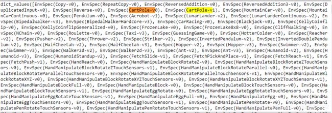
gym.envs.registry.all()

     The Cart-Pole is a very simple environment composed of a cart that can move left or right, and pole placed vertically on top of it. The agent must move the cart left or right to keep the pole upright.

create an environment with make()

env = gym.make('CartPole-v1')

After the environment is created, you must initialize it using the reset() method.. This returns an observation:

env.seed(42)
obs = env.reset()

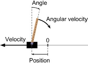
     Observations vary depending on the environment. In this case it is a 1D NumPy array composed of 4 floats: they represent the cart's horizontal position(0.0 = center), its velocity(positive means right), the angle of the pole (0 = vertical), and the angular velocity角速度(positive means clockwise).

obs

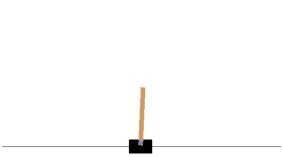
Figure 18-4. The CartPole environment 

     Here, we’ve created a CartPole environment. This is a 2D simulation in which a cart can be accelerated left or right in order to balance a pole placed on top of it (see Figure 18-4).

Now let’s display this environment by calling its render() method (see Figure 18-4) and and you can pick the rendering mode (the rendering options depend on the environment).. On Windows, this requires first installing an X Server, such as VcXsrv or Xming:

Warning: some environments (including the Cart-Pole) require access to your display, which opens up a separate window, even if you specify mode="rgb_array". In general you can safely ignore that window. However, if Jupyter is running on a headless server (ie. without a screen) it will raise an exception. One way to avoid this is to install a fake X server like Xvfb.

#########################################

On Debian or Ubuntu:

$ apt update
$ apt install -y xvfb

You can then start Jupyter using the xvfb-run command:

$ xvfb-run -s "-screen 0 1400x900x24" jupyter notebook

On google colab:

!apt-get install python-opengl -y
!apt install xvfb -y
!pip install pyvirtualdisplay
!pip install piglet
# !pip install gym

 you may to  Restart Runtime: then Run the above command again!

from IPython import display as ipythondisplay
from pyvirtualdisplay import Display

display = Display(visible=0, size=(1400, 900))
display.start()

#########################################

try:
    import pyvirtualdisplay
    display = pyvirtualdisplay.Display(visible=0, size=(1400, 900)).start()
except ImportError:
    pass


env.render()

 

If you want render() to return the rendered image as a NumPy array, you can set mode="rgb_array" (oddly, this environment will render the environment to screen as well):

img = env.render( mode='rgb_array' )
img.shape

def plot_environment( env, figsize=(5,4) ):
    plt.figure( figsize=figsize )
    img = env.render( mode="rgb_array" )
    plt.imshow( img )
    plt.axis("off")
    return img

import matplotlib.pyplot as plt
%matplotlib inline

plot_environment(env)
plt.show()

     Let's see how to interact with an environment. Your agent will need to select an action from an "action space" (the set of possible actions). Let's see what this environment's action space looks like:

env.action_space

 # action space
     Discrete(2) means that the possible actions are integers 0 and 1, which represent accelerating left (0) or right (1).

Other environments may have additional discrete actions, or other kinds of actions (e.g., continuous).

     Since the pole is leaning toward the right (obs[2] > 0, ), let’s accelerate the cart toward the right:

action = 1 # accelerate right
obs, reward, done, info = env.step( action )
obs

 

     Notice that (obs or observations)

• the cart's horizontal position(obs[0]< 0, 0.0 = center)
• the cart is now moving toward the right (obs[1] > 0，velocity (positive means right) ).
• The pole is still tilted toward the right (obs[2] > 0，the angle of the pole, 0 = vertical ),
• but its angular velocity is now negative (obs[3] < 0), so it will likely be tilted toward the left after the next step.

Figure 18-4. The CartPole environment 

The step() method executes the given action and returns four values:

• obs
  This is the new observation. The cart is now moving toward the right (obs[1] > 0). The pole is still tilted toward the right (obs[2] > 0), but its angular velocity is now negative (obs[3] < 0), so it will likely be tilted toward the left after the next step.
• reward
  In this environment, you get a reward of 1.0 at every step, no matter what you do, so the goal is to keep the episode running as long as possible.
• done
  This value will be True when the episode is over. This will happen when the pole tilts too much, or goes off the screen, or after 200 steps (in this last case, you have won). After that, the environment must be reset before it can be used again.
• info
  This environment-specific dictionary can provide some extra information that you may find useful for debugging or for training. For example, in some games it may indicate how many lives the agent has.

#######################
Once you have finished using an environment, you should call its close() method to free resources.
#######################

plot_environment( env )

Looks like it's doing what we're telling it to do!

The environment also tells the agent how much reward it got during the last step:

reward

When the game is over, the environment returns done=True:

done

     Finally, info is an environment-specific dictionary that can provide some extra information that you may find useful for debugging or for training. For example, in some games it may indicate how many lives the agent has.

info

     The sequence of steps between the moment the environment is reset until it is done is called an "episode". At the end of an episode (i.e., when step() returns done=True), you should reset the environment before you continue to use it.

if done:
    obs = env.reset()

     Now how can we make the pole remain upright? We will need to define a policy for that. This is the strategy that the agent will use to select an action at each step. It can use all the past actions and observations to decide what to do.

     Let’s hardcode a simple policy that accelerates left when the pole is leaning toward the left and accelerates right when the pole is leaning toward the right. We will run this policy to see the average rewards it gets over 500 episodes:

env.seed(42)

def plot_environment( env, figsize=(5,4) ):
    plt.figure( figsize=figsize )
    img = env.render( mode="rgb_array" )
    plt.imshow( img )
    plt.axis("off")
    return img

def basic_policy(obs):
    angle = obs[2]
    return 0 if angle<0 else 1 # possible actions are integers 0 and 1

totals=[]
for episode in range( 500 ):
    episode_rewards = 0
    obs = env.reset()
    # plot_environment( env )
    for step in range(200):
        action = basic_policy(obs)
        obs, reward, done, info = env.step( action ) # possible actions are integers 0 and 1
        # plot_environment( env )
        episode_rewards += reward
        
        if done:
            break
    totals.append( episode_rewards )

np.mean( totals ), np.std( totals ), np.min( totals ), np.max( totals )

This code is hopefully self-explanatory. Let’s look at the result: 

    Even with 500 tries, this policy never managed to keep the pole upright for more than 68 consecutive steps. Not great. If you look at the simulation in the Jupyter notebooks, you will see that the cart oscillates left and right more and more strongly until the pole tilts too much. Let’s see if a neural network can come up with a better policy.

Let's visualize one episode:

# Let's visualize one episode:

env.seed(42)

frames=[]

for step in range(200):
    img = env.render( mode='rgb_array' )
    frames.append(img)
    
    action = basic_policy( obs )
    obs, reward, done, info = env.step( action )
    
    if done:
        break
obs = env.reset() 

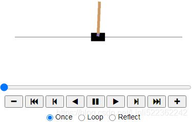
Now show the animation:

import matplotlib.animation as animation
import matplotlib as mpl
mpl.rc('animation', html='jshtml')

def update_scene( num, frames, patch ):
    patch.set_data( frames[num] )
    return patch,

def plot_animation( frames, repeat=False, interval=40 ):
    fig = plt.figure()
    patch = plt.imshow( frames[0] ) # img
    plt.axis( 'off' )
    
    anim = animation.FuncAnimation(
            fig,         # figure
            func=update_scene, # The function to call at each frame. 
            fargs=(frames, patch), # Additional arguments to pass to each call to func.
            frames = len(frames),  # iterable, int, generator function, or None, optional : Source of data to pass func and each frame of the animation
            repeat=repeat, 
            interval=interval
    )
    plt.close()
    return anim

plot_animation(frames)

 

Clearly the system is unstable and after just a few wobbles摇晃, the pole ends up too tilted: game over. We will need to be smarter than that!

Gym

env.observation_space

 

env.observation_space.shape[0]

 

env.observation_space.low

 

env.observation_space.high

 

obs

 

Neural Network Policies

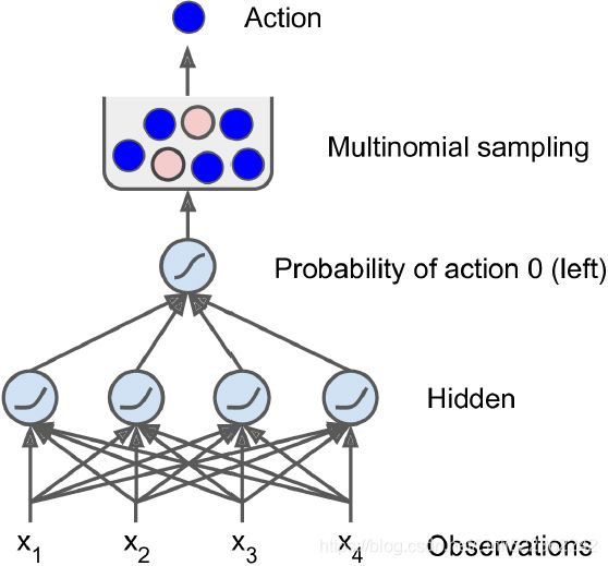Figure 18-5. Neural network policy

     Let’s create a neural network policy. Just like with the policy we hardcoded earlier, this neural network will take an observation as input, and it will output the action to be executed. More precisely, it will estimate a probability for each action, and then we will select an action randomly, according to the estimated probabilities (see Figure 18-5). In the case of the CartPole environment, there are just two possible actions (left or right), so we only need one output neuron. It will output the probability p of action 0 (left), and of course the probability of action 1 (right) will be 1 – p(==>keras.losses.binary_crossentropy). For example, if it outputs 0.7, then we will pick action 0 with 70% probability, or action 1 with 30% probability.

     You may wonder why we are picking a random action based on the probabilities given by the neural network, rather than just picking the action with the highest score. This approach lets the agent find the right balance between exploring new actions and exploiting[ɪkˈsplɔɪtɪŋ]利用；开拓,开发 the actions that are known to work well.(In general, exploitation will result in choosing actions with a greater short-term reward, whereas exploration can potentially result in greater total rewards in the long run.) Here’s an analogy: suppose you go to a restaurant for the first time, and all the dishes look equally appealing, so you randomly pick one. If it turns out to be good, you can increase the probability that you’ll order it next time, but you shouldn’t increase that probability up to 100%, or else you will never try out the other dishes, some of which may be even better than the one you tried.

     Also note that in this particular environment, the past actions and observations can safely be ignored, since each observation contains the environment’s full state. If there were some hidden state, then you might need to consider past actions and observations as well. For example,

• if the environment only revealed the position of the cart but not its velocity, you would have to consider not only the current observation but also the previous observation in order to estimate the current velocity.
• Another example is when the observations are noisy; in that case, you generally want to use the past few observations to estimate the most likely current state.
• The CartPole problem is thus as simple as can be; the observations are noise-free, and they contain the environment’s full state.

Here is the code to build this neural network policy using tf.keras:

from tensorflow import keras
import tensorflow as tf
import numpy as np

keras.backend.clear_session()
tf.random.set_seed(42)
np.random.seed(42)

# The number of inputs is the size of the observation space (which in the case of Cart‐Pole is 4)
n_inputs=4 # == env.observation_space.shape[0]

model = keras.models.Sequential([
    # input is obs including 4 features related to target action
    keras.layers.Dense(5, activation="elu", input_shape=[n_inputs]),
    keras.layers.Dense(1, activation="sigmoid"),
])

 Figure 18-5. Neural network policy

     After the imports, we use a simple Sequential model to define the policy network. The number of inputs is the size of the observation space (which in the case of Cart‐Pole is 4), and we have just five hidden units because it’s a simple problem. Finally, we want to output a single probability (the probability of going left), so we have a single output neuron using the sigmoid activation function. If there were more than two possible actions, there would be one output neuron per action, and we would use the softmax activation function instead.

Let's write a small function that will run the model to play one episode, and return the frames so we can display an animation:

def render_policy_net( model, n_max_steps=200, seed=42 ):
    frames = []
    env = gym.make("CartPole-v1")
    
    env.seed(seed)
    np.random.seed(seed)
    
    obs = env.reset()
    
    for step in range(n_max_steps):
        frames.append( env.render( mode="rgb_array" ) )
        # obs # the features related to target action
        # array([-0.01258566, -0.00156614,  0.04207708, -0.00180545])
        # obs.reshape(1,-1)
        # array([[-0.01258566, -0.00156614,  0.04207708, -0.00180545]])
        left_proba = model.predict( obs.reshape(1,-1) )
        action = int( np.random.rand() > left_proba )
        obs, reward, done, info = env.step( action )
        if done:
            break
    env.close()
    return frames

Now let's look at how well this randomly initialized policy network performs:

frames = render_policy_net( model )
plot_animation(frames)

Yeah... pretty bad. The neural network will have to learn to do better.

     First let's see if it is capable of learning the basic policy we used earlier: go left if the pole is tilting left, and go right if it is tilting right.

     We can make the same net play in 50 different environments in parallel (this will give us a diverse training batch at each step), and train for 5000 iterations. We also reset environments when they are done. We train the model using a custom training loop so we can easily use the predictions at each training step to advance the environments.
(n is input num_instances)==>divided by num_instances==>(m is input num_instances, n is num_features or input_dimensions) ==>tf.reduce_mean to get the average loss across 50 different environments
cp3 sTourOfMLClassifiers_stratify_bincount_likelihood_logistic regression_odds ratio_decay_L2_sigmoi_Linli522362242的专栏-CSDN博客

n_environments = 50
n_iterations = 5000

# make the same net play in 50 different environments in parallel
envs = [ gym.make("CartPole-v1") for _ in range( n_environments) ]

for index, env in enumerate( envs ):
    env.seed( index )
np.random.seed(42)

observations = [ env.reset() for env in envs ]

optimizer = keras.optimizers.RMSprop() # Nadam
loss_fn = keras.losses.binary_crossentropy # since the output is a single probability (the probability of going left

for iteration in range( n_iterations ):
    # We directly judge the next target action based on the current angle
    # if angle(or obs[2]) < 0, we want proba(going to left) = 1.
    # if angle > 0, we want proba(going to left) = 0.
    target_probas = np.array([ ( [1.] if obs[2]<0 else [0.] )
                              for obs in observations # 50 different environments in parallel ~ 50 groups of observations
                             ])
    
    with tf.GradientTape() as tape:
        # Based on the current observations, we predict the probability of the next action
        left_probas = model( np.array(observations) ) # Prediction: output the probability of going left
        # Improve predictions(to make the next predicted value is close to the target value) by minimizing the loss function
        # Use the gradient of the loss function to update the weights so that the next predicted value is close to the target value
        # The optimizer can speed up this process or reduce the steps required in the process

        # - np.log(sigmoid(z))     # if y=1
        # - np.log(1 - sigmoid(z)) # if y=0
        loss = tf.reduce_mean( loss_fn(target_probas, left_probas) ) # across 50 different environments
    print( "\rIteration: {}, Loss: {:.3f}".format( iteration, loss.numpy() ), 
           end="" 
         )
    grads = tape.gradient( loss, model.trainable_variables )
    optimizer.apply_gradients( zip(grads, model.trainable_variables) ) # training
    # select an action randomly for 50 environments seperately         
                # if () return true, then goes to right(1), otherwise, goes to left(0)
    actions = ( np.random.rand( n_environments, 1 ) > left_probas.numpy() ).astype( np.int32 )
    for env_index, env in enumerate( envs ):
        obs, reward, done, info = env.step( actions[env_index][0] )
        observations[env_index] = obs if not done else env.reset()
        # note ：env.reset() return obs: array([-0.02838569,  0.04781538,  0.0453429 , -0.03128895])
        
for env in envs:
    env.close()

frames = render_policy_net( model )
plot_animation( frames )

Looks like it learned the policy correctly. Now let's see if it can learn a better policy on its own. One that does not wobble as much(more wobbles 摇晃).

OK, we now have a neural network policy that will take observations and output action probabilities. But how do we train it?

Evaluating Actions: The Credit Assignment Problem

     If we knew what the best action was at each step, we could train the neural network as usual, by minimizing the cross entropy between the estimated probability distribution and the target probability distribution. It would just be regular supervised learning. However, in Reinforcement Learning the only guidance the agent gets is through rewards, and rewards are typically sparse and delayed. For example, if the agent manages to balance the pole for 100 steps, how can it know which of the 100 actions it took were good, and which of them were bad? All it knows is that the pole fell after the last action, but surely this last action is not entirely responsible. This is called the credit assignment problem: when the agent gets a reward, it is hard for it to know which actions should get credited (or blamed) for it. Think of a dog that gets rewarded hours after it behaved well; will it understand what it is being rewarded for?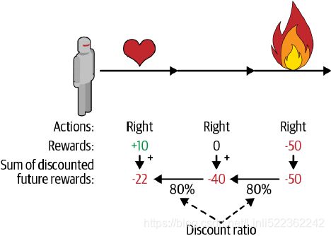
Figure 18-6. Computing an action’s return: the sum of discounted future rewards

     To tackle this problem, a common strategy is to evaluate an action based on the sum of all the rewards that come after it, usually applying a discount factor (gamma) at each step. This sum of discounted rewards is called the action’s return. Consider the example in Figure 18-6). If an agent decides to go right three times in a row and gets +10 reward after the first step, 0 after the second step, and finally –50 after the third step, then assuming we use a discount factor γ = 0.8, the first action will have a return of .

• If the discount factor is close to 0, then future rewards won’t count for much compared to immediate rewards. Conversely,
• if the discount factor is close to 1, then rewards far into the future will count almost as much as immediate rewards.
• Typical discount factors vary from 0.9 to 0.99. With a discount factor of 0.95, rewards 13 steps into the future count roughly for half as much as immediate rewards (since ≈ 0.5), while with a discount factor of 0.99, rewards 69 steps into the future count for half as much as immediate rewards(0.99^69≈0.5).

In the CartPole environment, actions have fairly short-term effects, so choosing a discount factor of 0.95 seems reasonable.

     Of course, a good action may be followed by several bad actions that cause the pole to fall quickly, resulting in the good action getting a low return (similarly, a good actor may sometimes star in a terrible movie). However, if we play the game enough times, on average good actions will get a higher return than bad ones. We want to estimate how much better or worse an action is, compared to the other possible actions, on average. This is called the action advantage. For this, we must run many episodes and normalize all the action returns (by subtracting the mean and dividing by the standard deviation). After that, we can reasonably assume that actions with a negative advantage were bad while actions with a positive advantage were good. Perfect—now that we have a way to evaluate each action, we are ready to train our first agent using policy gradients. Let’s see how.

Policy Gradients

     To train this neural network we will need to define the target probabilities y. If an action is good we should increase its probability, and conversely if it is bad we should reduce it. But how do we know whether an action is good or bad? The problem is that most actions have delayed effects, so when you win or lose points in an episode, it is not clear which actions contributed to this result: was it just the last action? Or the last 10? Or just one action 50 steps earlier? This is called the credit assignment problem.

     The Policy Gradients algorithm tackles this problem by first playing multiple episodes(step2), then making the actions in good episodes slightly more likely, while actions in bad episodes are made slightly less likely(step3). First we play, then we go back and think about what we did.

     As discussed earlier, PG algorithms optimize the parameters of a policy by following the gradients toward higher rewards. One popular class of PG algorithms, called REINFORCE algorithms, was introduced back in 1992 (Ronald J. Williams, “Simple Statistical Gradient-Following Algorithms for Connectionist Reinforcement Leaning,” Machine Learning 8 (1992) : 229–256.) by Ronald Williams. Here is one common variant:

• 1. First, let the neural network policy play the game several times, and at each step, compute the gradients that would make the chosen action even more likely—but don’t apply these gradients yet.
   
• step2. Once you have run several episodes, compute each action’s advantage (using the method described in the previous section).
   
• step3. If an action’s advantage is positive, it means that the action was probably good, and you want to apply the gradients computed earlier to make the action even more likely to be chosen in the future. However,
  
       if the action’s advantage is negative, it means the action was probably bad, and you want to apply the opposite gradients to make this action slightly less likely in the future. The solution is simply to multiply each gradient vector by the corresponding action’s advantage.
   
• 4. Finally, compute the mean of all the resulting gradient vectors, and use it to perform a Gradient Descent step.

     Let’s use tf.keras to implement this algorithm. We will train the neural network policy we built earlier so that it learns to balance the pole on the cart. First, we create a function to play a single step using the model. We will pretend for now that whatever action it takes is the right one so that we can compute the loss and its gradients (these gradients will just be saved for a while, and we will modify them later depending on how good or bad the action turned out to be):

def play_one_step( env, obs, model, loss_fn ):
    with tf.GradientTape() as tape:
        left_proba = model( obs[np.newaxis] ) # prediction
        # True/False = 1            # shape
        action = ( tf.random.uniform([1,1]) > left_proba ) # selection an action randomly
        y_target = tf.constant([ [1.] ]) # assume the y_target is 1: the cart goes to right
        loss = tf.reduce_mean( loss_fn(y_target, left_proba) )
        
    grads = tape.gradient( loss, model.trainable_variables )
    obs, reward, done, info = env.step( int( action[0,0].numpy() ) )
    return obs, reward, done, grads

Let’s walk though this function:

• • Within the GradientTape block (see Cp12 12 _Custom Models and Training with TensorFlow_2_progress_status_bar_Training Loops_concrete_tape_Linli522362242的专栏-CSDN博客), we start by calling the model, giving it a single observation (we reshape the observation so it becomes a batch containing a single instance, since the model expects a batch). This outputs the probability of going left.
   
• • Next, we sample a random float between 0 and 1, and we check whether it is greater than left_proba. The action will be False with probability left_proba, or True with probability 1 - left_proba.
  Once we cast this Boolean to a number, the action will be 0 (left) or 1 (right) with the appropriate probabilities.
   
• • Next, we define the target probability of going left: it is 1 minus the action (cast to a float). If the action is 0 (left), then the target probability of going left will be 1. If the action is 1 (right), then the target probability will be 0.
   
• • Then we compute the loss using the given loss function, and we use the tape to compute the gradient of the loss with regard to the model’s trainable variables. Again, these gradients will be tweaked later, before we apply them, depending on how good or bad the action turned out to be.
   
• • Finally, we play the selected action, and we return the new observation, the reward, whether the episode is ended or not, and of course the gradients that we just computed.

     Now let’s create another function that will rely on the play_one_step() function to play multiple episodes, returning all the rewards and gradients for each episode and each step:

def play_multiple_episodes( env, n_episodes, n_max_steps, model, loss_fn ):
    all_rewards = [] # n_episodes and 1 reward list per episode
    all_grads = []   # n_episodes and 1 gradient list per episode
    
    for episode in range( n_episodes ):
        current_rewards = [] # the number of steps <=n_max_steps and 1 reward per step
        current_grads = []   # the number of steps <=n_max_steps and 1 tuple of gradients per step
                             # each tuple containing 1 gradient tensor per trainable variable
        obs = env.reset()
        
        for step in range( n_max_steps ):
            obs, reward, done, grads = play_one_step( env, obs, model, loss_fn )
            current_rewards.append( reward ) # one reward per step
            current_grads.append( grads )    # 1 tuple of gradients per step, each tuple containing 1 gradient tensor per trainable variable
            if done:
                break
        all_rewards.append( current_rewards )
        all_grads.append( current_grads )
        
    return all_rewards, all_grads

# all_grads shape (episode_index, steps, variable_index]
     This code returns a list of reward lists (one reward list per episode, containing one reward per step), as well as a list of gradient lists (one gradient list per episode, each containing one tuple of gradients per step and each tuple containing one gradient tensor per trainable variable).

     The algorithm will use the play_multiple_episodes() function to play the game several times (e.g., 10 times), then it will go back and look at all the rewards, discount them, and normalize them. To do that, we need a couple more functions:

• the first will compute the sum of future discounted rewards at each step, and
   
• the second will normalize all these discounted rewards (returns) across many episodes by subtracting the mean and dividing by the standard deviation:

Let’s check that this works: 
  is the discount factor in range [0, 1]

     If an agent decides to go right three times in a row and gets +10 reward after the first step, 0 after the second step, and finally 50 after the third step, then assuming we use a discount factor γ = 0.8, the first action will have a return of 

import numpy as np

def discount_rewards( immediate_reward_list, discount_rate ):
  discounted = np.array( immediate_reward_list )
  # from back to front that to avoid use a recursion
  for reward_on_each_step in range( len(immediate_reward_list)-2, -1, -1 ):
    discounted[reward_on_each_step] += discounted[reward_on_each_step+1] * discount_rate
  return discounted

 The call to discount_rewards() returns exactly what we expect (see Figure 18-6). 

discount_rewards([10, 0, -50], discount_rate=0.8)

 

     Say there were 3 actions, and after each action there was a reward: first 10, then 0, then -50. If we use a discount factor of 80%, then

• the 3rd action will get -50 (full credit for the last reward), but
• the 2nd action will only get -40 (80% credit for the last reward), and
• the 1st action will get 80% of -40 (-32) plus full credit for the first reward (+10), which leads to a discounted reward of -22.

OR

 
     This means that the return at time t is equal to the immediate reward r plus the discounted future-return at time t + 1. This is a very important property, which facilitates the computations of the return.

def discounted_future_return( immediate_reward_list, discount_rate, index=0 ):
  immediate_reward_list = np.array(immediate_reward_list)

  if len(immediate_reward_list) ==1:
    return immediate_reward_list[0]

  if index == len(immediate_reward_list)-1 :
    return immediate_reward_list[index]

  # use a recursion
  return immediate_reward_list[index] + discount_rate * discounted_future_return( immediate_reward_list, discount_rate, index+1 )

discounted_future_return( [10, 0, -50], discount_rate=0.8, index=0 )

def discount_rewards( immediate_reward_list, discount_rate=0.8 ):
  discount_reward_list = []
  for index in range( len(immediate_reward_list) ): 
    discount_reward_list.append( discounted_future_return( immediate_reward_list, discount_rate, index ) )
  return discount_reward_list

discount_rewards([10, 0, -50], discount_rate=0.8)  

 

def discount_and_normalize_rewards( all_rewards, discount_rate ):
  all_discounted_rewards = [ discount_rewards( rewards, discount_rate )
                              for rewards in all_rewards ]
                          
  flat_rewards = np.concatenate( all_discounted_rewards ) # []+...[]=>[]
  reward_mean = flat_rewards.mean()
  reward_std = flat_rewards.std()

  return [ (discounted_rewards - reward_mean)/reward_std
           for discounted_rewards in all_discounted_rewards
         ]

discount_and_normalize_rewards( [ [10,0,-50], [10,20] ],
                                discount_rate=0.8
                              )

 To normalize all discounted rewards across all episodes, we compute the mean and standard deviation of all the discounted rewards, and we subtract the mean from each discounted reward, and divide by the standard deviation:

     You can verify that the function discount_and_normalize_rewards() does indeed return the normalized action advantages for each action in both episodes. Notice that the first episode was much worse than the second, so its normalized advantages are all negative; all actions from the first episode would be considered bad, and conversely all actions from the second episode would be considered good.

     We are almost ready to run the algorithm! Now let’s define the hyperparameters. We will run 150 training iterations, playing 10 episodes per iteration, and each episode will last at most 200 steps. We will use a discount factor of 0.95:

n_iterations = 150
n_episodes_per_update = 10 # playing 10 episodes per iteration
n_max_steps = 200
discount_rate = 0.95

     We also need an optimizer and the loss function. A regular Adam optimizer with learning rate 0.01 will do just fine, and we will use the binary cross-entropy loss function because we are training a binary classifier (there are two possible actions: left or right):

from tensorflow import keras

optimizer = keras.optimizers.Adam( learning_rate=0.01 )
loss_fn = keras.losses.binary_crossentropy

  

import tensorflow as tf

keras.backend.clear_session()
np.random.seed(42)
tf.random.set_seed(42)

model = keras.models.Sequential([
          keras.layers.Dense( 5, activation='elu', input_shape=[4] ),
          keras.layers.Dense( 1, activation='sigmoid' ),                                 
        ])

We are now ready to build and run the training loop!
##############

all_grads

all_grads[episode_index][step][var_index]
############## 

import  gym

env = gym.make( 'CartPole-v1' )
env.seed(42)

for iteration in range( n_iterations ): # n_iterations = 150
  all_rewards, all_grads = play_multiple_episodes(
                        env, n_episodes_per_update, n_max_steps, model, loss_fn
                        )
  total_rewards = sum( map(sum, all_rewards) )
  print('\rIteration: {}, mean rewards: {:.1f}'.format( iteration, 
                                                        total_rewards/n_episodes_per_update,
                                                        # end=""# show each iteration per row
                                                      ),
        end="" # show all iteration just on 1 row
       )
  all_final_rewards = discount_and_normalize_rewards( all_rewards,
                                                      discount_rate
                                                    )
  all_mean_grads = []
  # we compute the weighted mean of the gradients for that variable over all 
  # episodes and all steps, weighted by the final_reward.
  for var_index in range( len(model.trainable_variables) ):
    mean_grads = tf.reduce_mean( [final_reward * all_grads[episode_index][step][var_index]
                                  for episode_index, final_rewards in enumerate( all_final_rewards )
                                    for step, final_reward in enumerate(final_rewards)
                                 ], 
                                 axis=0
                               )
    all_mean_grads.append(mean_grads)
  optimizer.apply_gradients( zip(all_mean_grads, model.trainable_variables) )
  
env.close()

Let’s walk through this code:

• • At each training iteration, this loop calls the play_multiple_episodes() function, which plays the game 10 times and returns all the rewards and gradients for every episode and step.
   
• • Then we call the discount_and_normalize_rewards() to compute each action’s normalized advantage (which in the code we call the final_reward). This provides a measure of how good or bad each action actually was, in hindsight.
   
• • Next, we go through each trainable variable, and for each of them we compute the weighted mean of the gradients for that variable over all episodes and all steps, weighted by the final_reward.
• • Finally, we apply these mean gradients using the optimizer: the model’s trainable variables will be tweaked, and hopefully the policy will be a bit better.
  
  ... ...

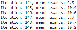
    And we’re done! This code will train the neural network policy, and it will successfully learn to balance the pole on the cart (you can try it out in the “Policy Gradients” section of the Jupyter notebook). The mean reward per episode will get very close to 160 (which is the maximum by default with this environment). Success!

frames = render_policy_net( model )
plot_animation(frames)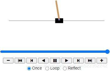

########################
    Researchers try to find algorithms that work well even when the agent initially knows nothing about the environment. However, unless you are writing a paper, you should not hesitate to inject prior knowledge into the agent, as it will speed up training dramatically. For example, since you know that the pole should be as vertical as possible, you could add negative rewards proportional to the pole’s angle. This will make the rewards much less sparse and speed up training. Also, if you already have a reasonably good policy (e.g., hardcoded), you may want to train the neural network to imitate it before using policy gradients to improve it.
########################

     The simple policy gradients algorithm we just trained solved the CartPole task, but it would not scale well to larger and more complex tasks. Indeed, it is highly sample inefficient, meaning it needs to explore the game for a very long time before it can make significant progress. This is due to the fact that it must run multiple episodes to estimate the advantage of each action, as we have seen. However, it is the foundation of more powerful algorithms, such as Actor-Critic algorithms (which we will discuss briefly at the end of this chapter).

    We will now look at another popular family of algorithms. Whereas PG algorithms directly try to optimize the policy to increase rewards, the algorithms we will look at now are less direct: the agent learns to estimate the expected return for each state, or for each action in each state, then it uses this knowledge to decide how to act. To understand these algorithms, we must first introduce Markov decision processes.

Markov Decision Processes

     In the early 20th century, the mathematician Andrey Markov studied stochastic processes with no memory, called Markov chains. Such a process has a fixed number of states, and it randomly evolves from one state to another at each step. The probability for it to evolve from a state s to a state s′ is fixed, and it depends only on the pair (s, s′), not on past states (this is why we say that the system has no memory).

Figure 18-7 shows an example of a Markov chain with four states.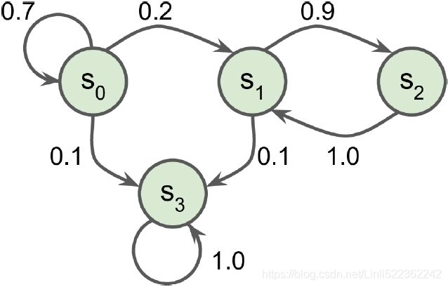Figure 18-7. Example of a Markov chain

    Suppose that the process starts in state , and there is a 70% chance that it will remain in that state at the next step. Eventually it is bound to leave that state and never come back because no other state points back to . If it goes to state , it will then most likely go to state (90% probability), then immediately back to state  (with 100% probability). It may alternate a number of times between these two states, but eventually it will fall into state and remain there forever (this is a terminal state). Markov chains can have very different dynamics, and they are heavily used in thermodynamics热力学, chemistry, statistics, and much more.

     Markov decision processes were first described in the 1950s by Richard Bellman.(Richard Bellman, “A Markovian Decision Process,” Journal of Mathematics and Mechanics 6, no. 5 (1957): 679–684.) They resemble Markov chains but with a twist: at each step, an agent can choose one of several possible actions, and the transition probabilities depend on the chosen action. Moreover, some state transitions return some reward (positive or negative), and the agent’s goal is to find a policy that will maximize reward over time.

     For example, the MDP represented in Figure 18-8 has three states (represented by circles)
and up to three possible discrete actions at each step (represented by diamonds).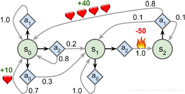
Figure 18-8. Example of a Markov decision process

     If it starts in state , the agent can choose between actions , , or .

• If it chooses action , it just remains in state with certainty, and without any reward. It can thus decide to stay there forever if it wants to.
• But if it chooses action , it has a 70% probability of gaining a reward of +10 and remaining in state . It can then try again and again to gain as much reward as possible, but at one point it is going to end up instead in state .

In state it has only two possible actions: or .

• It can choose to stay put by repeatedly choosing action ,
• or it can choose to move on to state and get a negative reward of –50 (ouch).

In state it has no other choice than to take action , which will most likely lead it back to state , gaining a reward of +40 on the way. You get the picture. By looking at this MDP, can you guess which strategy will gain the most reward over time? In state it is clear that action is the best option, and in state the agent has no choice but to take action , but in state it is not obvious whether the agent should stay put () or go through the fire ().

      Bellman found a way to estimate the optimal state value of any state s, noted V*(s), which is the sum of all discounted future rewards the agent can expect on average after it reaches a state s, assuming it acts optimally. He showed that if the agent acts optimally, then the Bellman Optimality Equation applies (see Equation 18-1). This recursive equation says that if the agent acts optimally, then the optimal value of the current state is equal to the reward it will get on average after taking one optimal action, plus the expected optimal value of all possible next states that this action can lead to.

Equation 18-1. Bellman Optimality Equation
 for all s 
OR cp18_Reinforcement Learning for Markov Decision Making in Env_Bellman_Q-learning_Q-Value Iteration_Linli522362242的专栏-CSDN博客

In this equation:

• • T(s, , s′) is the transition probability from state s to state s′, given that the agent chose action . For example, in Figure 18-8, = 0.8.
   
• • R(s, , s′) is the reward that the agent gets when it goes from state s to state s′, given that the agent chose action . For example, in Figure 18-8, R(s2, a1, s0) = +40.
   
• • γ is the discount factor.

    This equation leads directly to an algorithm that can precisely estimate the optimal state value of every possible state: you

• first initialize all the state value estimates to zero, and then you
• iteratively update them using the Value Iteration algorithm (see Equation 18-2).

A remarkable result is that, given enough time, these estimates are guaranteed to converge to the optimal state values, corresponding to the optimal policy.

Equation 18-2. Value Iteration algorithm for all s

OR 

 cp18_Reinforcement Learning for Markov Decision Making in Env_Bellman_Q-learning_Q-Value Iteration_Linli522362242的专栏-CSDN博客

 In this equation, is the estimated value of state s at the iteration of the algorithm.

     This algorithm is an example of Dynamic Programming, which breaks down a complex problem into tractable subproblems that can be tackled iteratively.

     Knowing the optimal state values can be useful, in particular to evaluate a policy, but it does not give us the optimal policy for the agent. Luckily, Bellman found a very similar algorithm to estimate the optimal state-action values, generally called Q-Values
(Quality Values). The optimal Q-Value of the state-action pair (s, a), noted Q*(s, ) OR , is the sum of discounted future rewards the agent can expect on average after it reaches the state s and chooses action , but before it sees the outcome of this action, assuming it acts optimally after that action. 

     Here is how it works: once again, you start by initializing all the Q-Value estimates to zero, then you update them using the Q-Value Iteration algorithm (see Equation 18-3).

Equation 18-3. Q-Value Iteration algorithm

     Once you have the optimal Q-Values, defining the optimal policy, noted π*(s) OR , is trivial: when the agent is in state s, it should choose the action  with the highest Q-Value for that state: .

     Let’s apply this algorithm to the MDP represented in Figure 18-8. First, we need to define the MDP:

Markov Chains

import numpy as np

np.random.seed(42)

transition_probabilities = [ # shape=[s, s']
                            [0.7, 0.2, 0.0, 0.1],  # from s0 to s0, s1, s2, s3
                            [0.0, 0.0, 0.9, 0.1],  # from s1 to ...
                            [0.0, 1.0, 0.0, 0.0],  # from s2 to ...
                            [0.0, 0.0, 0.0, 1.0]
                           ]  # from s3 to ...
n_max_steps = 50

def print_sequence():
  current_state = 0
  print( 'States:', end=' ')

  for step in range( n_max_steps ):
    print( current_state, end=' ' )
    if current_state == 3:
      break
    current_state = np.random.choice( range(4), 
                                      p=transition_probabilities[current_state]
                                    )
  else:
    print("...", end=" ")
  print()

for _ in range(10):
  print_sequence()

     Let's define some transition probabilities, rewards and possible actions. For example, in state s0, if action 0 is chosen then with proba 0.7 we will go to state s0 with reward +10, with probability 0.3 we will go to state s1 with no reward, and with never go to state s2 (so the transition probabilities are [0.7, 0.3, 0.0], and the rewards are [+10, 0, 0]):
==>

transition_probabilities = [# shape=[s, a, s']
                            #  s0 ,  s1,  s2 from s0
                            [ [0.7, 0.3, 0.0], # a0
                              [1.0, 0.0, 0.0], # a1
                              [0.8, 0.2, 0.0]  # a2
                            ],#s0 ,  s1,  s2 from s1
                            [ [0.0, 1.0, 0.0], # a0
                              None,            # a1
                              [0.0, 0.0, 1.0]  # a2 
                            ],#s0 ,  s1,  s2 from s2
                            [ None,            # a0
                              [0.8, 0.1, 0.1], # a1 
                              None             # a2
                            ]
                           ]
rewards = [ # shape=[s, a, s']
             # s0, s1, s2 from s0
            [ [+10, 0, 0], # a0
              [0, 0, 0],   # a1
              [0, 0, 0]    # a2
            ],#s0,s1,s2 from s1
            [ [0, 0, 0],   # a0
              [0, 0, 0],   # a1
              [0, 0, -50]  # a2
            ],#s0,s1,s2 from s2
            [ [0, 0, 0],   # a0
              [+40, 0, 0], # a1
              [0, 0, 0]    # a2
            ]
          ]
possible_actions = [ [0, 1, 2], # a0,a1,a2 for s0
                     [0, 2],    # a0,a2    for s1
                     [1]        # a1       for s2   
                   ]

import numpy as np

# In state s=1, it has only 2 possible action a=0 or a=2
# In state s=2, it has no other choice than to take action a=1
def policy_fire( state ): # action list : [0,2,1]
  return [0,2,1][state] # current state s=0 --> action a=0 -->s=1 -->a=2 --> s=2 --> a=1

def policy_safe( state ): # action list : [0,0,1]                       # x : path broken
  return [0,0,1][state] # current state s=0 --> action a=0 -->s=1 -->a=0 -x-> s=2 --> a=1    

def policy_random( state ):
  return np.random.choice( possible_actions[state] )

class MDPEnvironment( object ):
  def __init__( self, start_state=0 ):
    self.start_state = start_state
    self.reset()

  def reset( self ):
    self.total_rewards = 0
    self.state = self.start_state

  def step( self, action ):
    # Generate a non-uniform(given p) random sample from range(3) of size 1:
    next_state = np.random.choice( range(3),
                                   p = transition_probabilities[self.state][action]
                                 )
    reward = rewards[self.state][action][next_state]
    self.state = next_state
    self.total_rewards += reward

    return self.state, reward

def run_episode( policy, n_steps, start_state=0, display=True ):
  env = MDPEnvironment()
  if display:
    print( "States (+rewards):", end=" " )

  for step in range( n_steps ):
    if display: 
      if step == 10: # only print state within 10 steps
        print( "...", end=" " )
      elif step < 10:
        print( env.state, end=" " )
      
    action = policy( env.state )
    state, reward = env.step( action )

    if display and step < 10:
      if reward:
        print( "({})".format(reward), end=" " )

  if display:
    print( "Total rewards =", env.total_rewards )
    
  return env.total_rewards

for policy in ( policy_fire, policy_random, policy_safe ):
  all_totals = []
  print( policy.__name__)
  np.random.seed(42)
  env.seed(42)

  for episode in range( 1000 ):
    all_totals.append( run_episode( policy, n_steps=100, display=(episode<5) ) )
 
  print( "Summary about rewards: mean={:.1f}, std={:1f}, min={}, max={}".format(
                                 np.mean( all_totals ),
                                 np.std( all_totals ),
                                 np.min( all_totals ),
                                 np.max( all_totals )
                              )
       )  
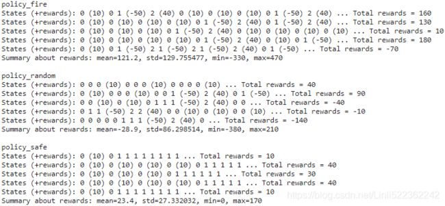
  print()

 policy_fire is perfect and action list : [0,2,1] for state s=[0,1,2]

     For example, to know the transition probability from s2 to s0 after playing action 1, we will look up transition_probabilities[2][1][0] (which is 0.8). Similarly, to get the corresponding reward, we will look up rewards[2][1][0] (which is +40). And to get the list of possible actions in s2, we will look up possible_actions[2] (in this case, only action a1 is possible). Next, we must initialize all the Q-Values to 0 (except for the the impossible actions, for which we set the Q-Values to –∞):

Q_values = np.full( (3,3), 
                    fill_value = -np.inf # -np.inf for impossible actions
                  )
for state, actions in enumerate( possible_actions ):
  Q_values[state, actions] = 0.0  # for all possible actions

     Now let’s run the Q-Value Iteration algorithm. It applies Equation 18-3 repeatedly,(the +1 iteration) to all Q-Values, for every state and every possible action:

Q-Value Iteration

Dynamic programming
     In this section, we will focus on solving RL problems under the following assumptions:

• • We have full knowledge about the environment dynamics; that is, all transition probabilities (′, ′|, ) are known.
• • The agent's state has the Markov property, which means that the next action and reward only depend on the current state and the choice of action we make at this moment or current time step

https://blog.csdn.net/Linli522362242/article/details/117889535

gamma = 0.90 # the discount factor

history1 = []

for iteration in range(50):
  Q_prev = Q_values.copy()
  history1.append( Q_prev )

  for s in range(3):
    for a in possible_actions[s]:
      Q_values[s,a] = np.sum([ transition_probabilities[s][a][next_s]
                               * ( rewards[s][a][next_s] + gamma*np.max( Q_prev[next_s] )
                                 )
                               for next_s in range(3)
                             ]
                            )
history1 = np.array( history1 )

 That’s it! The resulting Q-Values look like this:

Q_values

 

     For example, when the agent is in state s0 and it chooses action a1, the expected sum of discounted future rewards is approximately 17.0( Q(s, ) ).

     For each state, let’s look at the action that has the highest Q-Value(Q(s, )):

np.argmax(Q_values, axis=1)

  # policy_safe

     This gives us the optimal policy for this MDP, when using a discount factor of 0.90:

• in state s0 choose action a0;
• in state s1 choose action a0 (i.e., stay put); and
• in state s2 choose action a1 (the only possible action).

Interestingly, if we increase the discount factor to 0.95, the optimal policy changes: in state s1 the best action becomes a2 (go through the fire!).

gamma = 0.95 # the discount factor

history1 = []

for iteration in range(50):
  Q_prev = Q_values.copy()
  history1.append( Q_prev )

  for s in range(3):
    for a in possible_actions[s]:
      Q_values[s,a] = np.sum([ transition_probabilities[s][a][next_s]
                               * ( rewards[s][a][next_s] + gamma*np.max( Q_prev[next_s] )
                                 )
                               for next_s in range(3)
                             ]
                            )
np.argmax(Q_values, axis=1)

 # policy_fire

    This makes sense because the more you value future rewards, the more you are willing to put up with some pain now for the promise of future bliss[blɪs]未来的幸福. ( This is because the discount factor is larger so the agent values the future more, and it is therefore ready to pay an immediate penalty in order to get more future rewards.==>) 

Temporal Difference Learning

     Reinforcement Learning problems with discrete actions can often be modeled as Markov decision processes, but the agent initially has no idea what the transition probabilities are (it does not know T(s, a, s′)), and it does not know what the rewards are going to be either (it does not know R(s, a, s′)). It must experience each state and each transition at least once to know the rewards, and it must experience them multiple times if it is to have a reasonable estimate of the transition probabilities.

     The Temporal Difference Learning (TD Learning) algorithm is very similar to the Value Iteration algorithm, but tweaked to take into account the fact that the agent has only partial knowledge of the MDP(Markov Decision Processes). In general we assume that the agent initially knows only the possible states and actions, and nothing more. The agent uses an exploration policy—for example, a purely random policy—to explore the MDP, and as it progresses, the TD Learning algorithm updates the estimates of the state values based on the transitions and rewards that are actually observed (see Equation 18-4).

Equation 18-4. TD Learning algorithm( the +1 iteration of the algorithm)

 or, equivalently:
 OR

In this equation:

• • α is the learning rate (e.g., 0.01), which is kept constant during learning.
• • is called the TD target. OR
• • is called the TD error.

     A more concise way of writing the first form of this equation is to use the notation , which means . So, the first line of Equation 18-4 can be rewritten like this: .

    TD Learning has many similarities with Stochastic Gradient Descent, in particular the fact that it handles one sample at a time. Moreover, just like Stochastic GD, it can only truly converge if you gradually reduce the learning rate (otherwise it will keep bouncing around the optimum Q-Values).

    For each state s, this algorithm simply keeps track of a running average of the immediate
rewards the agent gets upon leaving that state, plus the rewards it expects to get later (assuming it acts optimally).

Q-Learning

    Similarly, the Q-Learning algorithm is an adaptation of the Q-Value Iteration algorithm to the situation where the transition probabilities and the rewards are initially unknown (see Equation 18-5). Q-Learning works by watching an agent play (e.g., randomly) and gradually improving its estimates of the Q-Values. Once it has accurate Q-Value estimates (or close enough), then the optimal policy is choosing the action that has the highest Q-Value (i.e., the greedy policy).

Equation 18-5. Q-Learning algorithm

     For each state-action pair (s, a), this algorithm keeps track of a running average of the rewards r the agent gets upon leaving the state s with action a, plus the sum of discounted future rewards it expects to get. To estimate this sum, we take the maximum of the Q-Value estimates for the next state s′, since we assume that the target policy would act optimally from then on.

     Let’s implement the Q-Learning algorithm. First, we will need to make an agent explore the environment. For this, we need a step function so that the agent can execute one action and get the resulting state and reward:

import numpy as np

def step( state, action ):
  probas = transition_probabilities[state][action]
  next_state = np.random.choice( [0,1,2], 
                                 p = probas
                               )
  reward = rewards[state][action][next_state]
  return next_state, reward

    Now let’s implement the agent’s exploration policy. Since the state space is pretty small, a simple random policy will be sufficient. If we run the algorithm for long enough, the agent will visit every state many times, and it will also try every possible action many times:

def exploration_policy( state ):
  return np.random.choice( possible_actions[state] )

    Next, after we initialize the Q-Values just like earlier, we are ready to run the QLearning algorithm with learning rate decay (using power scheduling, introduced in Chapter 11 11_Training Deep Neural Networks_3_Adam_Learning Rate Scheduling_Decay_np.argmax(」)_lambda语句_Regular_Linli522362242的专栏-CSDN博客):

np.random.seed( 42 )

Q_values = np.full( (3,3), -np.inf )
for state, actions in enumerate( possible_actions ):
  Q_values[state][actions] = 0

Q_values

 

• Power scheduling
  
  Set the learning rate to a function of the iteration number t (#I believe t is steps in keras#): η(t) = . The initial learning rate , the power c (typically set to 1), and the steps s (#I believe s is decay_steps in keras#) are hyperparameters.
  https://blog.csdn.net/Linli522362242/article/details/107086444
• Q-Value Iteration
• Q-learning replaces V with Q in formula

alpha0 = 0.05 # initial learning rate
decay = 0.005 # learning rate decay
gamma = 0.90  # discount factor
state = 0 # initial rate
history2 = []

for iteration in range( 10000 ):
  history2. append( Q_values.copy() )
  action = exploration_policy( state )

  next_state, reward = step( state, action )
  next_state_Q_value = np.max( Q_values[next_state] ) # greedy policy at the next step

  # Power scheduling
  # https://blog.csdn.net/Linli522362242/article/details/107086444
  alpha = alpha0 / ( 1 + iteration*decay )

  Q_values[state, action] *= 1-alpha
  Q_values[state, action] += alpha * ( reward + gamma*next_state_Q_value )
  state = next_state

history2 = np.array( history2 )

Q_values

 

np.argmax( Q_values, axis=1 )

 

import matplotlib.pyplot as plt

# history1 shape: (50,3,3)
true_Q_value = history1[-1][0][0] # -1 : last iteration
                                  # 0 : state_0
                                  # 0 : action_0 

fig, axes = plt.subplots( 1,2, figsize=(10,4), sharey=True )

axes[0].set_ylabel( "Q-Value$(s_0, a_0)$", fontsize=14 )
axes[0].set_title( "Q-Value Iteration", fontsize=14 )

axes[1].set_title( "Q-Learning", fontsize=14 )
                                     # iterations
for ax, width, history in zip( axes, (50,10000), (history1, history2) ):

  ax.plot( [0, width], [true_Q_value, true_Q_value], "k--" )
  # history1[:,0,0] : TypeError: list indices must be integers or slices, not tuple
  # since history: [array([[]]), ..., array([[]])]
  history= np.array(history)
  ax.plot( np.arange(width), history[:,0,0], "b-", linewidth=2 )

  ax.set_xlabel('Iterations', fontsize=14)
  ax.axis( [0, width, 0, 24] )

 Figure 18-9. The Q-Value Iteration algorithm (left) versus the Q-Learning algorithm(right)

      This algorithm will converge to the optimal Q-Values, but it will take many iterations(10000), and possibly quite a lot of hyperparameter tuning. As you can see in Figure 18-9, the Q-Value Iteration algorithm (left) converges very quickly(total 50 iteration), in fewer than 20 iterations, while the Q-Learning algorithm (right) takes about 8,000 iterations to converge. Obviously, not knowing the transition probabilities or the rewards makes finding the optimal policy significantly harder!

     The Q-Learning algorithm is called an off-policy algorithm because the policy being trained is not necessarily the one being executed因为被训练的策略不一定是正在执行的策略: in the previous code example, the policy being executed (the exploration policy) is completely random,

def exploration_policy( state ):
  return np.random.choice( possible_actions[state] )

while the policy being trained will always choose the actions with the highest Q-Values. ###next_state_Q_value = np.max( Q_values[next_state] ) # greedy policy at the next step### Conversely, the Policy Gradients algorithm is an on-policy algorithm: it explores the world using the policy being trained. It is somewhat surprising that Q-Learning is capable of learning the optimal policy by just watching an agent act randomly (imagine learning to play golf when your teacher is a drunk monkey). Can we do better?

 Exploration Policies

    Of course, Q-Learning can work only if the exploration policy explores the MDP thoroughly enough. Although a purely random policy is guaranteed to eventually visit every state and every transition many times, it may take an extremely long time to do so. Therefore, a better option is to use the ε-greedy policy (ε is epsilon): at each step it acts randomly with probability ε, or greedily with probability 1–ε (i.e., choosing the action with the highest Q-Value). The advantage of the ε-greedy policy (compared to a completely random policy) is that it will spend more and more time exploring the interesting parts of the environment, as the Q-Value estimates get better and better, while still spending some time visiting unknown regions of the MDP. It is quite common to start with a high value for ε (e.g., 1.0) and then gradually reduce it (e.g., down to 0.05).

     Alternatively, rather than relying only on chance for exploration, another approach is to encourage the exploration policy to try actions that it has not tried much before. This can be implemented as a bonus added to the Q-Value estimates, as shown in Equation 18-6.

 Equation 18-6. Q-Learning using an exploration function

 In this equation:

• • N(s′, a′) counts the number of times the action a′ was chosen in state s′.
   
• • f(Q, N) is an exploration function, such as f(Q, N) = Q + κ/(1 + N), where κ is a curiosity hyperparameter that measures how much the agent is attracted to the unknown.

 Approximate Q-Learning and Deep Q-Learning

 Ms. Pac-Man (see Figure 18-1)

Colab 

import urllib.request
urllib.request.urlretrieve('http://www.atarimania.com/roms/Roms.rar','Roms.rar')
!pip install unrar
!unrar x Roms.rar
!mkdir rars
!mv HC\ ROMS.zip   rars
!mv ROMS.zip  rars
!python -m atari_py.import_roms rars

import gym
import pyvirtualdisplay
display = pyvirtualdisplay.Display(visible=0, size=(1400, 900)).start()

# Next we will load the MsPacman environment, version 0.
env = gym.make('MsPacman-v0')

# Let's initialize the environment by calling is reset() method. This returns an observation:
env.seed(42)
obs = env.reset()

obs.shape

 Observations vary depending on the environment. In this case it is an RGB image represented as a 3D NumPy array of shape [width, height, channels] (with 3 channels: Red, Green and Blue). In other environments it may return different objects, as we will see later.

# In this example we will set mode="rgb_array" to get an image of the environment as a NumPy array:
img = env.render( mode="rgb_array" )

import matplotlib.pyplot as plt

plt.figure( figsize=(5,4) )
plt.imshow( img )
plt.axis( "off" )

plt.show()

     The main problem with Q-Learning is that it does not scale well to large (or even medium) MDPs with many states and actions. For example, suppose you wanted to use Q-Learning to train an agent to play Ms.Pac-Man吃豆人(see Figure 18-1).There are about 150 pellets['pelɪt]颗粒 that Ms. Pac-Man can eat, each of which can be present or absent (i.e., already eaten). So, the number of possible states is greater than 2^150 ≈ 10^45. And if you add all the possible combinations of positions for all the ghosts and Ms. Pac-Man, the number of possible states becomes larger than the number of atoms in our planet, so there’s absolutely no way you can keep track of an estimate for every single Q-Value.

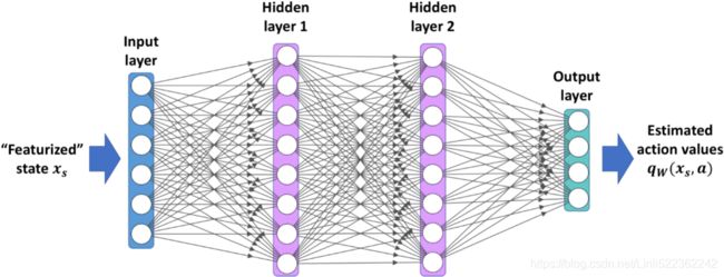
    The solution is to find a function that approximates the Q-Value of any state-action pair (s, a) using a manageable number of parameters (given by the parameter vector θ). This is called Approximate Q-Learning. For years it was recommended to use linear combinations of handcrafted features extracted from the state (e.g., distance of the closest ghosts, their directions, and so on) to estimate Q-Values, but in 2013, DeepMind showed that using deep neural networks can work much better, especially for complex problems, and it does not require any feature engineering. A DNN used to estimate Q-Values is called a Deep Q-Network (DQN), and using a DQN for Approximate Q-Learning is called Deep Q-Learning.

     Now, how can we train a DQN? Well, consider the approximate Q-Value computed by the DQN for a given state-action pair (s, a). Thanks to Bellman, we know we want this approximate Q-Value to be as close as possible to the reward r that we actually observe after playing action a in state s, plus the discounted value of playing optimally from then on.
     To estimate this sum of future discounted rewards, we can simply execute the DQN on the next state s′ and for all possible actions a′. We get an approximate future Q-Value for each possible action. We then pick the highest (since we assume we will be playing optimally) and discount it, and this gives us an estimate of the sum of future discounted rewards. By summing the reward r and the future discounted value estimate, we get a target Q-Value y(s, a) for the state-action pair (s, a), as shown in Equation 18-7.

Equation 18-7. Target Q-Value

     With this target Q-Value, we can run a training step using any Gradient Descent algorithm.
Specifically, we generally try to minimize the squared error between the estimated Q-Value Q(s, a) and the target Q-Value (or the Huber loss to reduce the algorithm’s sensitivity to large errors). And that’s all for the basic Deep Q-Learning algorithm! Let’s see how to implement it to solve the CartPole environment.

Implementing Deep Q-Learning

     The first thing we need is a Deep Q-Network. In theory, you need a neural net that takes a state-action pair and outputs an approximate Q-Value, but in practice it’s much more efficient to use a neural net that takes a state and outputs one approximate Q-Value for each possible action. To solve the CartPole environment, we do not need a very complicated neural net; a couple of hidden layers will do:

import tensorflow as tf
from tensorflow import keras
import numpy as np
import gym

keras.backend.clear_session()
tf.random.set_seed(42)
np.random.seed(42)

env = gym.make("CartPole-v1")
input_shape = [4] # == env.observation_space.shape # states
n_outputs = 2     # == env.action_space.n          # number of actions, move to left or right

model = keras.models.Sequential([
            keras.layers.Dense( 32, activation="elu", input_shape = input_shape),
            keras.layers.Dense( 32, activation="elu" ),
            keras.layers.Dense( n_outputs )
          ])
# e.g. uses the DQN to predict the Q-Value for each possible action in each experience’s next state.

    To select an action using this DQN, we pick the action with the largest predicted Q-Value. To ensure that the agent explores the environment, we will use an ε-greedy policy (i.e., we will choose a random action with probability ε):

def epsilon_greedy_policy( state, epsilon=0 ):
  if np.random.rand() < epsilon:
    # OR
    # return np.random.choice(n_outputs) 
    # OR
    # import random.randrange(2)
    # random.randrange()
    return np.random.randint( n_outputs )
  else:
    Q_values = model.predict( state[np.newaxis] )# ==>(batch_size, input_shape)
    return np.argmax( Q_values[0] ) # maximum of Q_values at current state ~ action(goes to left or right)

     Instead of training the DQN based only on the latest experiences, we will store all experiences in a replay buffer (or replay memory, in the form of tuples: (obs, action, reward, next_obs, done).), and we will sample a random training batch from it at each training iteration. This helps reduce the correlations between the experiences in a training batch, which tremendously helps training. For this, we will just use a deque list(We can use the deque class for that (but make sure to check out DeepMind's excellent Reverb library for a much more robust implementation of experience replay)):

• self.memory = deque( maxlen = max_memory_size )
• self.memory.append( transition ) # transition: (s, a, r, next_s, done)
• https://blog.csdn.net/Linli522362242/article/details/117889535

Implementing the replay memory

     The replay memory can be implemented using a Python list, where every time we add a new element to the list, we need to check the size of the list and call pop(0) if needed.

     Alternatively, we can use the deque data structure from the Python collections library, which allows us to specify an optional argument, max_len. By specifying the max_len argument, we will have a bounded deque. Therefore, when the object is full, appending a new element results in automatically removing an element from it.

     Note that this is more efficient than using a Python list, since removing the first element of a list using pop(0) has O(n) complexity, while the deque's runtime complexity is O(1). You can learn more about the deque implementation from the official documentation that is available at https://docs.python.org/3.7/library/collections.html#collections.deque.

     A deque is a linked list, where each element points to the next one and to the previous one. It makes inserting and deleting items very fast, but the longer the deque is, the slower random access will be. If you need a very large replay buffer, use a circular buffer; 

Deque vs Rotating List

The deque class offers fast append, but fairly slow random access (for large replay memories):

from collections import deque
import numpy as np

np.random.seed(42)

mem = deque( maxlen=1000000)
for i in range( 1000000 ):
  mem.append(i)

[ mem[i] for i in np.random.randint(1000000, size=5) ]

%timeit mem.append(1)

    The slowest run took 25.10 times longer than the fastest. This could mean that an intermediate result is being cached这可能意味着正在缓存中间结果. 10000000 loops, best of 5: 76.9 ns per loop

%timeit [ mem[i] for i in np.random.randint(1000000, size=5) ]

     Alternatively, you could use a rotating list like this ReplayMemory class. This would make random access faster for large replay memories:

class ReplayMemory:
  def __init__( self, max_size ):
    self.buffer = np.empty( max_size, dtype=np.object )
    self.max_size = max_size
    self.index = 0
    self.size = 0
  
  def append( self, obj ):
    self.buffer[ self.index ] = obj
    self.size = min( self.size+1, self.max_size )
    self.index = ( self.index+1 ) % self.max_size

  def sample( self, batch_size ):
    indices = np.random.randint( self.size, size=batch_size )
    return self.buffer[ indices ]

mem = ReplayMemory( max_size=1000000 )
for i in range( 1000000 ):
  mem.append( i )
mem.sample( 5 )

 

%timeit mem.append(1)

%timeit mem.sample(5)

 ###########################

from collections import deque

replay_memory = deque( maxlen=2000 )

     Each experience will be composed of five elements: a state, the action the agent took, the resulting reward, the next state it reached, and finally a Boolean indicating whether the episode ended at that point (done). We will need a small function to sample a random batch of experiences from the replay buffer. It will return 5 NumPy arrays corresponding to the 5 experience elements:

def sample_experiences( batch_size ):
  indices = np.random.randint( len(replay_memory), size=batch_size )
  batch = [ replay_memory[index] for index in indices ]
  # [ [states], [actions], [rewards], [next_states], [dones] ]
  states, actions, rewards, next_states, dones = [ np.array([ experience[field_index] 
                                                              for experience in batch
                                                            ])
                                                   for field_index in range(5)
                                                 ]
  return states, actions, rewards, next_states, dones 

     Let’s also create a function that will use the DQN to play a single step using the ε-greedy policy, then store the resulting experience in the replay buffer:

def play_one_step( env, state, epsilon ):
  action = epsilon_greedy_policy( state, epsilon )
  next_state, reward, done, info = env.step( action )
  replay_memory.append( (state, action, reward, next_state, done) )
  return next_state, reward, done, info

     Finally, let’s create one last function that will sample a batch of experiences from the replay buffer and train the DQN by performing a single Gradient Descent step on this batch:

 Equation 18-7. Target Q-Value

batch_size = 32
discount_rate = 0.95
optimizer = keras.optimizers.Adam( learning_rate=1e-2 )
loss_fn = keras.losses.mean_squared_error

def training_step( batch_size ):

  experiences = sample_experiences( batch_size )
  states, actions, rewards, next_states, dones = experiences

  next_Q_values = model.predict( next_states )
  # Q_values shape: (states, actions)
  max_next_Q_values = np.max( next_Q_values, axis=1 )
  target_Q_values = ( rewards + 
                      (1-dones)*discount_rate*max_next_Q_values
                    ) # note: if dones=True ==>int(True)=1, then target_Q_values=rewards
  target_Q_values = target_Q_values.reshape(-1,1)
  # e.g. actions [1, 1, 0, ...] ==>  [[0, 1], [0, 1], [1, 0],...] 
  mask = tf.one_hot( actions, n_outputs )

  with tf.GradientTape() as tape:
    all_Q_values = model( states )
    Q_values = tf.reduce_sum( all_Q_values * mask, # zero out all the Q-Values we do not want
                              axis = 1,
                              keepdims = True
                            ) # sum over axis 1 to get rid of all the zeros,
                           # MSE 
    loss = tf.reduce_mean( loss_fn( target_Q_values, Q_values )
                         )# ==>minimize: mse([[target_Q_value],...]-[[Q_values],...])
  grads = tape.gradient( loss, model.trainable_variables )
  optimizer.apply_gradients( zip(grads, model.trainable_variables) )

 Let’s go through this code:

• • First we define some hyperparameters, and we create the optimizer and the loss function.
   
• • Then we create the training_step() function. It starts by sampling a batch of experiences, then it uses the DQN to predict the Q-Value for each possible action in each experience’s next state. Since we assume that the agent will be playing optimally, we only keep the maximum Q-Value for each next state. Next, we use Equation 18-7 to compute the target Q-Value for each experience’s state-action pair.
   
• • Next, we want to use the DQN to compute the Q-Value for each experienced state-action pair. However, the DQN will also output the Q-Values for the other possible actions, not just for the action that was actually chosen by the agent. So we need to mask out all the Q-Values we do not need. The tf.one_hot() function makes it easy to convert an array of action indices into such a mask. For example, if the first three experiences contain actions 1, 1, 0, respectively, then the mask will start with [[0, 1], [0, 1], [1, 0],...]. We can then multiply the DQN’s output with this mask, and this will zero out all the Q-Values we do not want. We then sum over axis 1 to get rid of all the zeros, keeping only the QValues of the experienced state-action pairs. This gives us the Q_values tensor, containing one predicted Q-Value for each experience in the batch.
   
• • Then we compute the loss: it is the mean squared error between the target and predicted Q-Values for the experienced state-action pairs.
• • Finally, we perform a Gradient Descent step to minimize the loss with regard to the model’s trainable variables.

This was the hardest part. Now training the model is straightforward:

env.seed(42)
np.random.seed(42)
tf.random.set_seed(42)
keras.backend.clear_session()

rewards = []
best_score = 0

for episode in range( 600 ):
  obs = env.reset()

  for step in range( 200 ):
    epsilon = max( 1-episode/500, 0.01 )
    obs, reward, done, info = play_one_step( env, obs, epsilon )
    if done:
      break
  
  rewards.append( step )

  # Current Return >= Current largest return
  if step >= best_score:
    best_weights = model.get_weights()
    best_score = step
    print( "\rEpisode: {}, Steps: {}, eps: {:.3f}".format( episode, step+1, epsilon ), 
          end="" )
  # The reason we play 50 episodes without training is to give the replay buffer 
  # some time to fill up (if we don’t wait enough, then there will not be enough 
  # diversity in the replay buffer  
  if episode > 50:
    training_step( batch_size )

model.set_weights( best_weights )  

     We run 600 episodes, each for a maximum of 200 steps. At each step,

• we first compute the epsilon value for the ε-greedy policy: it will go from 1 down to 0.01, linearly, in a bit under 500 episodes. # epsilon = max( 1-episode/500, 0.01 )
   
• Then we call the play_one_step() function, which will use the ε-greedy policy to pick an action, then execute it and record the experience( Transition(state, action, reward, next_state, done) ) in the replay buffer.
   
• If the episode is done, we exit the loop.
   
• Policy Improvement using the idea of , ( if step(Current Return) >= best_score(Current largest return), then update model weights )
   
• Finally, if we are past the 50th episode, we call the training_step() function to train the model on one batch sampled from the replay buffer. The reason we play 50 episodes without training is to give the replay buffer some time to fill up (if we don’t wait enough, then there will not be enough diversity in the replay buffer). And that’s it, we just implemented the Deep Q-Learning algorithm!

import matplotlib.pyplot as plt

plt.figure(figsize=(8, 4))
plt.plot(rewards)
plt.xlabel("Episode", fontsize=14)
plt.ylabel("Sum of rewards", fontsize=14)

plt.show()

Figure 18-10 shows the total rewards the agent got during each episode. 

Figure 18-10. Learning curve of the Deep Q-Learning algorithm 

     As you can see, the algorithm made may no apparent progress没有明显的进展 at all for almost 300 episodes (in part because ε was very high at the beginning), then at some point, its performance suddenly skyrocketed up to 200 (which is the maximum possible performance in this environment). That’s great news: the algorithm worked fine, and it actually ran much faster than the Policy Gradient algorithm! But wait… just a few episodes later, it forgot everything it knew, and its performance dropped below 50! This is called catastrophic forgetting灾难性遗忘, and it is one of the big problems facing virtually all RL algorithms: as the agent explores the environment, it updates its policy, but what it learns in one part of the environment may break what it learned earlier in other parts of the environment. The experiences are quite correlated, and the learning environment keeps changing—this is not ideal for Gradient Descent!

• If you increase the size of the replay buffer, the algorithm will be less subject to this problem.如果增加重放缓冲区的大小，算法将较少受此问题的影响.
• Reducing the learning rate may also help.

But the truth is, Reinforcement Learning is hard: training is often unstable, and you may need to try many hyperparameter values and random seeds before you find a combination that works well. For example, if you try changing the number of neurons per layer in the preceding from 32 to 30 or 34, the performance will never go above 100 (the DQN may be more stable with one hidden layer instead of two).

     Reinforcement Learning is notoriously difficult, largely because of the training instabilities and the huge sensitivity to the choice of hyperparameter values and random seeds.(A great 2018 post by Alex Irpan nicely lays out RL’s biggest difficulties and limitations.)As the researcher Andrej Karpathy put it: “[Supervised learning] wants to work. […] RL must be forced to work.” You will need time, patience, perseverance, and perhaps a bit of luck too. This is a major reason RL is not as widely adopted as regular Deep Learning (e.g., convolutional nets). But there are a few real-world applications, beyond AlphaGo and Atari games: for example, Google uses RL to optimize its datacenter costs, and it is used in some robotics applications, for hyperparameter tuning, and in recommender systems.

     You might wonder why we didn’t plot the loss. It turns out that loss is a poor indicator of the model’s performance.

• The loss might go down, yet the agent might perform worse (e.g., this can happen when the agent gets stuck in one small region of the environment, and the DQN starts overfitting this region).
• Conversely, the loss could go up, yet the agent might perform better (e.g., if the DQN was underestimating the Q-Values, and it starts correctly increasing its predictions, the agent will likely perform better, getting more rewards, but the loss might increase because the DQN also sets the targets, which will be larger too).

     The basic Deep Q-Learning algorithm we’ve been using so far would be too unstable to learn to play Atari games. So how did DeepMind do it? Well, they tweaked the algorithm!

Deep Q-Learning Variants

18_2Reinforcement Learning_\r_end=““_Deep Q-Learning_Double DQN_Dueling DQN_TF-Agents_Linli522362242的专栏-CSDN博客