基于逻辑回归(Logistic Regression)的糖尿病视网膜病变(Diabetic Retinopathy)检测
基于逻辑回归的糖尿病视网膜病变检测
- 说明
-
- 数据集
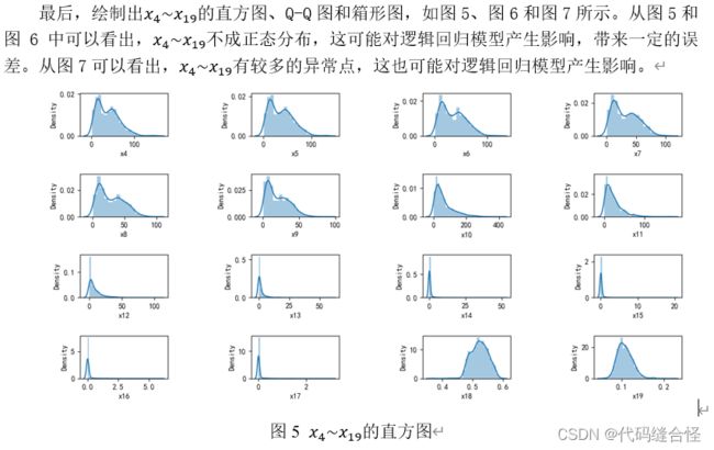
- 探索性数据分析
- 方法
- 结果
- 代码
说明
这是我学机器学习的一个项目, 基于逻辑回归(Logistic Regression)的糖尿病视网膜病变(Diabetic Retinopathy)检测 ,该模型采用机器学习中逻辑回归的方式,训练Diabetic Retinopathy Debrecen Data Set的数据集,获得模型参数,建立预测模型,可以有效针对DR疾病做出预测和分类。仅供参考,莫要抄袭!!!
数据集
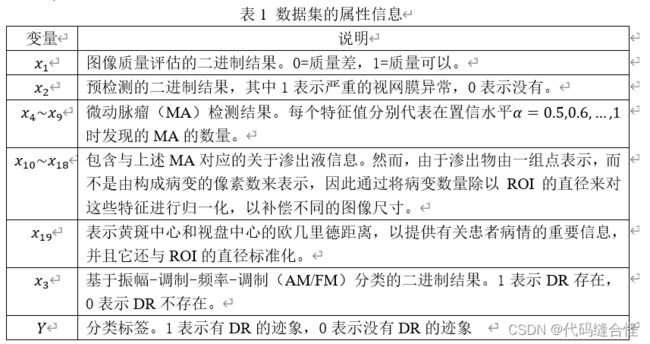
该数据集是从UCI机器学习库下载的,并且该数据集包含了从Messidor图像集中提取的19个特征,可用于预测图像是否有糖尿病视网膜病变(DR)的迹象,详细信息如表1所示。数据集下载链接:
https://archive.ics.uci.edu/ml/datasets/Diabetic+Retinopathy+Debrecen+Data+Set
探索性数据分析
首先,分析第1类特征(变量x1, x2, x3)。分别绘制变量x1, x2, x3和Y的交叉报表,如表2、表3和表4所示。从表2和表3可以计算出,x1=1的占比为1147/1151≈99.7%,x2=1的占比为1057/1151≈91.8% 。对于变量x3,x3=1表示DR存在,x3=0表示DR不存在,和实际值Y对比,计算出准确率为(347+194)/1151≈47.0%.
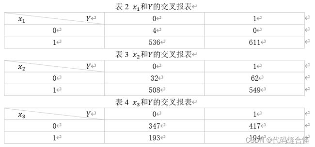
因此,在Messidor图像集中,99.7%的图片的质量可以,能够用来训练逻辑回归模型,91.8%的图片预检测有严重的视网膜异常,而AM/FM的预测结果准确率只有47.0%,准确率偏低,所以变量x1, x2, x3并没有提供有用的信息。
方法
数据标准化
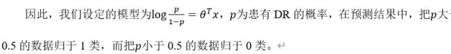
 逻辑回归
逻辑回归
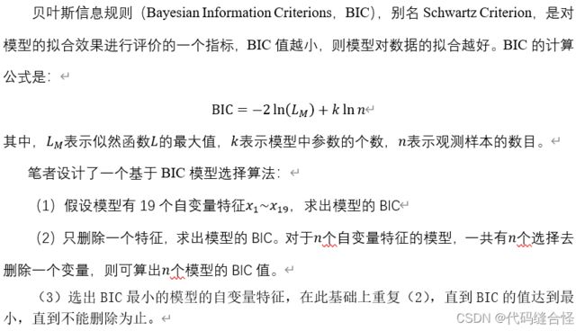
 模型选择
模型选择
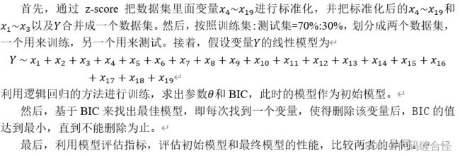
 整体方案
整体方案
结果
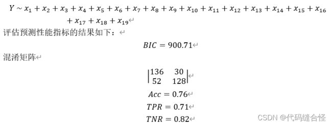
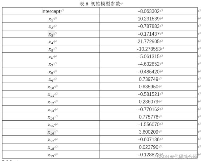
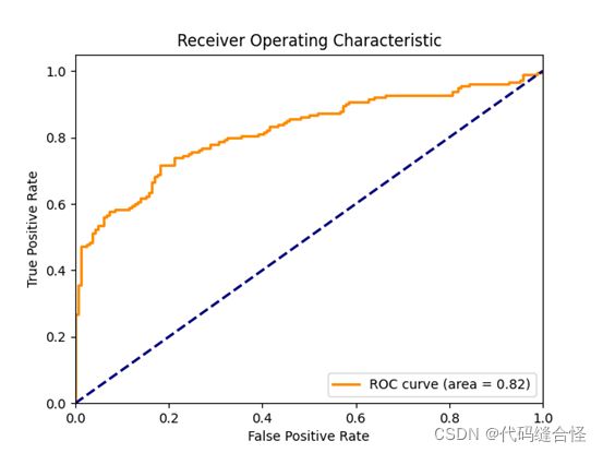
初始模型

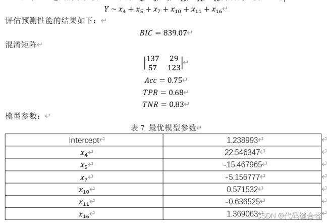
 最终模型
最终模型
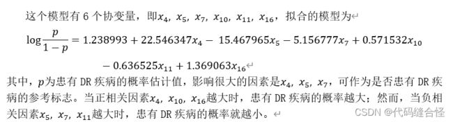
 总结
总结
代码
数据分析
import pandas as pd
import seaborn as sns
import numpy as np
import matplotlib.pyplot as plt
from scipy.io import arff
from scipy.stats import norm

# pycharm控制台输出显示pandas设置
pd.set_option('display.max_columns', 1000)
pd.set_option('display.width', 1000)
pd.set_option('display.max_colwidth', 1000)
# plt显示中文
plt.rcParams['font.sans-serif'] = ['SimHei']  # 配置字体,显示中文
plt.rcParams['axes.unicode_minus'] = False  # 配置坐标轴刻度值模式,显示负号

# 导入数据
df = arff.loadarff("../homework_2/messidor_features.arff")
print(df)
data = pd.DataFrame(df[0])
Cnames = ['x1', 'x2', 'x4', 'x5', 'x6', 'x7', 'x8', 'x9', 'x10', 'x11', 'x12', 'x13',
          'x14', 'x15', 'x16', 'x17', 'x18', 'x19', 'x3', 'y']
# x1, x2, and x3 are binary
data.columns = Cnames
print("data:\n", data.head())
print("shape:", data.shape)
print("统计:\n", data.describe())

data.replace('N/A', np.NAN, inplace=True)
print(data.isnull().any())  # 判断数据集每一列是否有缺失值
print(data.isnull().sum(axis=0))  # 求出每一列对应的缺失值的个数

print("每一列数值统计: \n")
for col in Cnames:
    print(data[col].value_counts(), end="\n\n")


# a. 2进制变量的条形图:x1,x2,x3,y
sets = ['x1', 'x2', 'x3']
for col in sets:
    temp = pd.crosstab(data.loc[:, col], data.y)
    print(temp, "\n\n")
    ax = temp.plot(kind='bar', grid=True, title=col+'-y')
    ax.set_xlabel(col)
    ax.set_ylabel(col+" count")
    plt.show()


# b. 相关系数的热力图
# cor = data[['x4', 'x5', 'x6', 'x7', 'x8', 'x9', 'x10', 'x11', 'x12', 'x13',
#             'x14', 'x15', 'x16', 'x17', 'x18', 'x19']].corr()
cor = data[['x10', 'x11', 'x12', 'x13', 'x14', 'x15', 'x16', 'x17', 'x18', 'x19']].corr()
print("相关系数矩阵:\n", cor)
sns.heatmap(cor, cmap='GnBu', annot=True, fmt='.2f',
            linewidths=0.1, vmin=-1, vmax=1)
plt.show()


# c. x4-x19的箱形图
sets = ['x4', 'x5', 'x6', 'x7', 'x8', 'x9', 'x10', 'x11',
        'x12', 'x13', 'x14', 'x15', 'x16', 'x17', 'x18', 'x19']
sns.boxplot(data=data[sets])
plt.show()
sns.boxenplot(data=data[sets])  # 增强型
plt.show()
sns.stripplot(data=data[sets], jitter=True)  # 散点图, 散点左右"抖动"效果
plt.show()

# d. x4-x19的直方图
i = 1
for col in sets:
    data1 = data.loc[:, col]
    plt.subplot(4, 4, i)
    sns.distplot(data1)
    i += 1
plt.tight_layout()  # 自动调整子图参数,使得子图不重叠
plt.show()

# e.Q-Q plot
i = 1
for col in sets:
    data1 = data.loc[:, col]
    prob = (np.arange(data1.shape[0]) - 1 / 2) / data1.shape[0]
    q = norm.ppf(prob, 0, 1)
    y = data1.to_numpy()
    y = (y - np.mean(y)) / np.std(y)
    y.sort()
    plt.subplot(4, 4, i)
    plt.scatter(x=q, y=y, color='red', s=1)
    plt.plot(y, y, color='blue')  # Add a 45-degree reference line
    plt.xlabel(col)
    i += 1
plt.tight_layout()  # 自动调整子图参数,使得子图不重叠
plt.show()
数据训练
import pandas as pd
import numpy as np
import matplotlib.pyplot as plt
from scipy.io import arff
from sklearn import preprocessing
from sklearn.model_selection import train_test_split
import statsmodels.api as sm
from sklearn.metrics import confusion_matrix, roc_curve, auc

# pycharm控制台输出显示pandas设置
pd.set_option('display.max_columns', 1000)
pd.set_option('display.width', 1000)
pd.set_option('display.max_colwidth', 1000)

# 导入数据集
df = arff.loadarff("../homework_2/messidor_features.arff")
data = pd.DataFrame(df[0])
Cnames = ['x1', 'x2', 'x4', 'x5', 'x6', 'x7', 'x8', 'x9', 'x10', 'x11', 'x12', 'x13',
          'x14', 'x15', 'x16', 'x17', 'x18', 'x19', 'x3', 'y']
data.columns = Cnames  # x1, x2, and x3 are binary
print("data:\n", data.head())
print("shape:", data.shape)

# 数据预处理
x = data.iloc[:, 2:data.shape[1] - 2].astype('float32')
print('before z-score:\n', x)
# z-score 标准化 x
std_scaler = preprocessing.StandardScaler()
x = std_scaler.fit_transform(x)
x = pd.DataFrame(x, columns=Cnames[2:data.shape[1] - 2])
print('after z-score:\n', x)
# 合并
Data = pd.concat([data['x1'].astype('int'), data['x2'].astype('float32'), x, data['x3'].astype('float32'), data['y'].astype('float32')], axis=1)
print('before split:\n', Data)

# 划分测试集和训练集
train_data, test_data = train_test_split(Data, train_size=0.7, random_state=120)
print('after split:\n', train_data)

# 寻找最优训练方法
method_group = []
formula = "y ~ x1+x2+x3+x4+x5+x6+x7+x8+x9+x10+x11+x12+x13+x14+x15+x16+x17+x18+x19"
methods = ['newton', 'bfgs', 'lbfgs', 'powell', 'cg', 'ncg', 'basinhopping', 'minimize']
for method in methods:
    model = sm.Logit.from_formula(formula, data=train_data)
    re1 = model.fit(method=method)
    method_group.append((method, np.round(re1.bic, 2)))
method_group.sort(key=lambda x:x[1], reverse=False)  # 从小到大排序
print(method_group)

# 训练
formula = "y ~ x1+x2+x3+x4+x5+x6+x7+x8+x9+x10+x11+x12+x13+x14+x15+x16+x17+x18+x19"
model = sm.Logit.from_formula(formula, data=train_data)
re1 = model.fit(method='ncg')
print(re1.summary())

print("AIC = ", np.round(re1.aic, 2))
print("BIC = ", np.round(re1.bic, 2))
# 可以返回变量的边际效应和对应的置信区间
print(re1.get_margeff(at="overall").summary())


# 评估

# 1.混淆矩阵
y_test = test_data.y
y_pred = re1.predict(test_data)
cut_off = 0.5
y_pred[y_pred >= cut_off] = 1
y_pred[y_pred < cut_off] = 0
print("confusion_matrix:\n", confusion_matrix(y_test, y_pred))

# 2.ROC曲线
tn, fp, fn, tp = confusion_matrix(y_test, y_pred).ravel()
predicted_values = re1.predict(test_data)
fpr, tpr, thresholds = roc_curve(y_test, predicted_values)
roc_auc = auc(fpr, tpr)
lw = 2
plt.plot(fpr, tpr, color='darkorange', lw=lw,
         label='ROC curve (area = %0.2f)' % roc_auc)  # 假正率为横坐标,真正率为纵坐标做曲线
plt.plot([0, 1], [0, 1], color='navy', lw=lw, linestyle='--')
plt.xlim([0.0, 1.0])
plt.ylim([0.0, 1.05])
plt.xlabel('False Positive Rate')
plt.ylabel('True Positive Rate')
plt.title('Receiver Operating Characteristic')
plt.legend(loc="lower right")
plt.show()

# 3.准确率、TPR、TNR
accuracy = (tn+tp)/(tn+fp+fn+tp)
print("Accuracy = ", np.round(accuracy, 2))
TPR = tp/(tp+fn)
TNR = tn/(tn+fp)
print("TPR = ", np.round(TPR, 2))
print("TNR = ", np.round(TNR, 2))

# 输出模型参数
coef = re1.params  # 逻辑回归模型参数 pd.Series
print(coef)
coef_list = []
for i in np.arange(len(coef)):
    coef_list.append((coef.index[i], np.round(coef[i], 3)))
coef_list.sort(key=lambda x:x[1], reverse=True)  # 将参数从大到小排序
print(coef_list)


# 模型选择
def model_selection(data):  # data: DataFrame
    col_names = list(data.columns)[:-1]
    BIC = []
    AIC = []
    formula = 'y ~ ' + ' + '.join(list(data.columns)[:-1])
    model = sm.Logit.from_formula(formula, data=data)
    re1 = model.fit(method='ncg')
    AIC.append(('Full Model', np.round(re1.aic, 2)))
    BIC.append(('Full Model', np.round(re1.bic, 2)))
    for i in range(len(col_names)):
        c = list(data.columns)[:-1]
        c.pop(i)
        formula = 'y ~ ' + ' + '.join(c)
        model = sm.Logit.from_formula(formula, data=data)
        re1 = model.fit(method='ncg')
        AIC.append((col_names[i], np.round(re1.aic, 2)))
        BIC.append((col_names[i], np.round(re1.bic, 2)))
        AIC.sort(key=lambda x:x[1])  # 将AIC从小到大排序
        BIC.sort(key=lambda x:x[1])  # 将BIC从小到大排序
    return AIC, BIC


# 基于BIC选择模型:每次找到一个变量,使得删除变量后,AIC和BIC的值达到最小,直到不能剔除为止
flag = 0
feature_drop = []  # 删除的特征
while flag == 0:
    AIC, BIC = model_selection(train_data)
    if BIC[0][0] == 'Full Model':
        break
    else:
        feature_drop.append(BIC[0][0])
        train_data.drop(BIC[0][0], axis=1, inplace=True)
        test_data.drop(BIC[0][0], axis=1, inplace=True)
print(feature_drop)  # 删除的特征
print(Cnames[0:-1])  # 所有的特征

# 最终模型
fal_formula = 'y ~ '
for ch in Cnames[0:-1]:
    if ch not in feature_drop:
        fal_formula = fal_formula + ch + '+'
fal_formula = fal_formula[0:-1]
print(fal_formula)  # 最终模型表达式


# 最终模型的训练
model = sm.Logit.from_formula(fal_formula, data=train_data)
re1 = model.fit(method='ncg')
print(re1.summary())
print("AIC = ", np.round(re1.aic, 2))
print("BIC = ", np.round(re1.bic, 2))
print(re1.get_margeff(at="overall").summary())


# 评估

# 1.混淆矩阵
y_test = test_data.y
y_pred = re1.predict(test_data)
cut_off = 0.5
y_pred[y_pred >= cut_off] = 1
y_pred[y_pred < cut_off] = 0
print("confusion_matrix:\n", confusion_matrix(y_test, y_pred))

# 2.ROC曲线
tn, fp, fn, tp = confusion_matrix(y_test, y_pred).ravel()
predicted_values = re1.predict(test_data)
fpr, tpr, thresholds = roc_curve(y_test, predicted_values)
roc_auc = auc(fpr, tpr)
lw = 2
plt.plot(fpr, tpr, color='darkorange', lw=lw,
         label='ROC curve (area = %0.2f)' % roc_auc)  # 假正率为横坐标,真正率为纵坐标做曲线
plt.plot([0, 1], [0, 1], color='navy', lw=lw, linestyle='--')
plt.xlim([0.0, 1.0])
plt.ylim([0.0, 1.05])
plt.xlabel('False Positive Rate')
plt.ylabel('True Positive Rate')
plt.title('Receiver Operating Characteristic')
plt.legend(loc="lower right")
plt.show()

# 3.准确率、TPR、TNR
accuracy = (tn+tp)/(tn+fp+fn+tp)
print("Accuracy = ", np.round(accuracy, 2))
TPR = tp/(tp+fn)
TNR = tn/(tn+fp)
print("TPR = ", np.round(TPR, 2))
print("TNR = ", np.round(TNR, 2))

# 输出模型参数
coef = re1.params  # 逻辑回归模型参数 pd.Series
print(coef)
coef_list = []
for i in np.arange(len(coef)):
    coef_list.append((coef.index[i], np.round(coef[i], 3)))
coef_list.sort(key=lambda x:x[1], reverse=True)  # 将参数从大到小排序
print(coef_list)