生成对抗方式解决医学图像重建 Adversarially learned iterative reconstruction for imaging inverse problems

Introduction

Problem description

In the area of medical image reconstruction, we want to recover $x^{\ast }\in \mathbb{X}$ containing critic information in the polar coordinate from data
$y=\mathcal{A}\left(x^{\ast }\right)+e\in \mathbb{Y}$, which exert a transform like the Randon Transforms to original data with noise $e\in \mathbb{Y}$,and often demonstrated in a sinogram. Both the forward operator and the distribution of the noise are typically known. Yet the inverse problem are always ill-posed,meaning that there’re more than one parameters for model due to inadequate information of measurement and we cannot recover precisely the original image.

Reserch overview

traditional method to tackle the inverse problem is variational reconstruction, combining the Euclidean distance and a regularizer.

${\min }_{\mathbf{x}\in \mathbb{X}}\Vert \mathbf{y}-\mathcal{A}(\mathbf{x}){\Vert }_2^2+\lambda \mathcal{R}(\mathbf{x})$

the regularizer is effective by penalizing unlikely solutions and restore prior knowledge about the image.

With the development of DL,data-driven methods are proposed，and can be classified as follows：

• end-to-end over parameterized models,which need large amount of paired examples
• learn a regularizer encoding prior knowledge of image by networks and apply it to reconstruction tasks

Yet, all of them are faced with problems like difficulty in obtaining data, overfitting, poor genalization ability in unseen data and high computational expenses

Main contribution

loss function

Instead of training the reconstruction model in a supervised way that we train it with paired training examples $\{x_i,y_i{\}}_{i=1}^N$ ,we propose an unsupervised method based on probabilistic models on X and Y and evaluate the reconstruction quality by the wasserstein distance $\mathcal{W}\left({\left({\mathcal{G}}_{\theta }\right)}_{\#}{\pi }_Y,{\pi }_X\right)$.The wasserstein distance is defined as $W_p(\mu ,\nu )={\left({\inf }_{\gamma \in \Gamma (\mu ,\nu )}{\mathbf{E}}_{(x,y)\sim \gamma }d(x,y{)}^p\right)}^{1/p}$. It can measure thedifferent of two distribution and take their geometric characteristics into account. In this way,we not necessarily need paired examples for training. We take advantage of the wasserstein distance for our regularizer. Moreover, ${\mathcal{G}}_{\theta }$should be approximate to both right-inverse and left-inverse of forward operator $\mathcal{A}$.

$\begin{array}{rlr}J(\theta )=\mathcal{W}\left({\left({\mathcal{G}}_{\theta }\right)}_{\#}{\pi }_Y,{\pi }_X\right)+{\lambda }_{\mathbb{Y}}{\mathbb{E}}_{{\pi }_Y}[& {\Vert \mathcal{A}\left({\mathcal{G}}_{\theta }(Y)\right)-Y\Vert }_2^2]& +{\lambda }_{\mathbb{X}}{\mathbb{E}}_{{\pi }_X}\left[{\Vert {\mathcal{G}}_{\theta }(\mathcal{A}(X))-X\Vert }_2^2\right]\end{array}$

When we implement the training the model, we make use of the Kantorovich-Rubinstein (KR) duality for approximating the wasserstein distance (proof) as:

$$\mathcal{L}(\mathcal{R})={\mathbb{E}}_{{\pi }_X}[\mathcal{R}(X)]-{\mathbb{E}}_{{\pi }_Y}\left[\mathcal{R}\left({\mathcal{G}}_{\theta }(Y)\right)\right]$$where$$\underset{\mathcal{R}}{\inf }\mathcal{L}(\mathcal{R})=-\mathcal{W}\left({\left({\mathcal{G}}_{\theta }\right)}_{\#}{\pi }_Y,{\pi }_X\right)$$or simplified as$$\mathcal{W}\left({\left({\mathcal{G}}_{\theta }\right)}_{\#}{\pi }_Y,{\pi }_X\right)=\sup {\mathbb{E}}_{{\pi }_X}\left[{\mathcal{D}}_{\alpha }(X)\right]-{\mathbb{E}}_{{\left({\mathcal{G}}_{\theta }\right)}_{\#}{\pi }_Y}\left[{\mathcal{D}}_{\alpha }(X)\right]\text{ where }{\mathcal{D}}_{\alpha }\in {\mathbb{L}}_1\text{. }$$

In this sense, we set a descriminator in the GAN as a regularizer aiming at maximize the accuracy of desciminating a sample from ${\pi }_X$ and ${\pi }_Y$，wherein the 1-Lipschitz condition is enforced by penalizing the gradient of the critic network $({{\Vert \nabla {\mathcal{D}}_{\alpha }\left(\mathbf{x}\right)\Vert }_2-1)}^2$
From maximum-likehood perspective,except for the measurement of different distribution, the loss function reminiscent the tractable evidence lower-bound (ELBO) of the maximum-likehood
${\max }_{\theta }\left[\frac{1}{n_1}{\sum }_{i=1}^{n_1}\log {\pi }_X^{(\theta )}\left({\mathbf{x}}_i\right)+\frac{1}{n_2}{\sum }_{i=1}^{n_2}\log {\pi }_Y^{(\theta )}\left({\mathbf{y}}_i\right)\right]$

denoted by

${\min }_{\theta }KL\left({\pi }_{X\mid Y=\mathbf{y}}^{(r)},{\pi }_X\right)+\frac{1}{2{\sigma }_e^2}{\Vert \mathbf{y}-\mathcal{A}\left({\mathcal{G}}_{\theta }(\mathbf{y})\right)\Vert }_2^2+\frac{1}{2{\sigma }_2^2}{\Vert \mathbf{x}-{\mathcal{G}}_{\theta }(\mathcal{A}(\mathbf{x}))\Vert }_2^2$

Parameterizing the model

Learned primal-dual algorithm

The architecture of ${\mathcal{G}}_{\theta }$ is built upon the idea of iterative unrolling(seminal work), and adopt the learned primal-dual algorithm, which is proposed to solve wide range of inverse problems ${\min }_{f\in X}[\mathcal{F}(\mathcal{K}(f))+\mathcal{G}(f)]$.

As $\mathcal{G}$ is typically non-smooth, an proximal operator defined by ${\mathrm{prox}}_{\tau \mathcal{G}}(f)=\underset{f^{\prime }\in X}{\mathrm{argmin}}\left[\mathcal{G}\left(f^{\prime }\right)+\frac{1}{2\tau }{\Vert f^{\prime }-f\Vert }_X^2\right]$ is employed, which is regarded as extensive form of gradient descent. Conjugate function has good properties, so it is used to induce a primal dual hybrid gradient to achieve the optimal goal ${\min }_x{\max }_y\mathcal{G}(x)+⟨y,\mathcal{K}x⟩-{\mathcal{F}}^{\ast }(y)$ . The optimality condition is
$$\{\begin{array}{l}0\in \partial \mathcal{G}(x)+\partial \mathcal{K}(x{)}^{T}y\\ 0\in \mathcal{K}(x)-\partial {\mathcal{F}}^{\ast }(y)\end{array}$$
Through fixed point iteration, a non-linear primal dual hybrid gradient method is proposed to solve the problem.And considering the covergence of the algorithm, it also gives initialization constraints.

In data driven deep learning method, all of the parameters including proximal operator $prox$,step length $\sigma$ and $\tau$ , overrelaxation parameter $\gamma$ are learned through deep neural network. The architecture of the model follows the scheme of iterative alternating update.

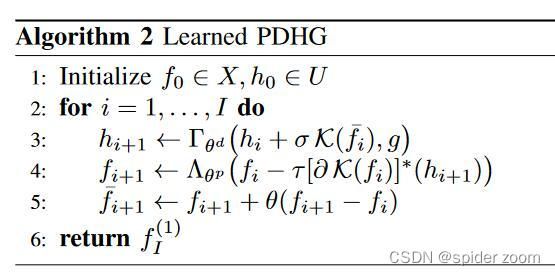
The Learned Primal-Dual model is trained using a learning rate scheme according to cosine annealing ${\eta }_t=\frac{{\eta }_0}{2}\left(1+\cos \left(\pi \frac{t}{t_{\max }}\right)\right)$.The paper also gives modifications to the model that allow it to combine previous iterative result to obtain the learned result by extend the dual (and primal) space from $U$ to $U^{N_{dual}}$.

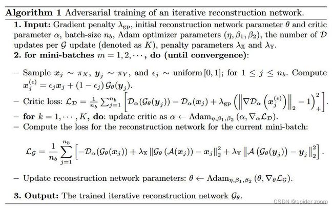
algorithm proposed

Reconstruction network and critic network are established and they’re trained in an adversarial and alternating way. First, model parameters, including critic network parameters and reconstruction parameters,max iterations,penalty parameters,are set as the input. Then we sample original data and measured data from respecive marginal distributions ,and train critic network and update critic parameters for $k$ times. Finally we train reconstruction network and update reconstruction parameters for once.

Following the settings in the Learned PDHG,the reconstruction model ${\mathcal{G}}_{\theta }$ is conputed by applying ${\mathbf{h}}^{(\ell +1)}={\Gamma }_{{\theta }_d^{(\ell )}}\left({\mathbf{h}}^{(\ell )},{\sigma }^{(\ell )}\mathcal{A}\left({\mathbf{x}}^{\ell }\right),\mathbf{y}\right)$ and ${\mathbf{x}}^{(\ell +1)}={\Lambda }_{{\theta }_{\mathrm{p}}^{(\ell )}}\left({\mathbf{x}}^{(\ell )},{\tau }^{(\ell )}{\mathcal{A}}^{\ast }\left({\mathbf{h}}^{\ell +1}\right)\right)$ for $L$ times and ${\mathbf{h}}^{(0)}=0$, ${\mathbf{x}}^{(0)}$ is the filtered back projection(FBP) reconstruction. The critic model ${\mathcal{D}}_{\alpha }$ is simply a feed-forward CNN with four cascaded layer.

Numerical results and conclusion

We consider sparse CT reconstruction,classical inverse problem.We generate a set of 2000 2D phantoms containing 5 ellipses placed randomly, each of which has density chosen uniformly at random in the range [0.1,1]. Another dataset consisting of 2250 2D slices extracted from human abdominal CT scans. We conduct comparision study of ALPD with state-of-art model-driven and data-driven methods like FBP,LPD and TV.We take PSNR, SSIM, running time and number of parameters as comparision indicators, and we also evaluate reconstruction visually and compare their texture details.We draw conclusions as below.

• ALPD performs almost identical to the total-variation (TV) method in terms of reproduce the ellipses area delineated by sharp boundaries, and well discern the small tumors, outperforming LPD.
• ALPD is superior to LPD in recovering clinically important features, since it does well in delineation.
• ALPD have less parameters than AR TV, and FBP+UNet, so it may need less scale dataset. ALPD performs similar to LPD in running time, PSNR and SSIM, but it can be trained against unsupervised data.

References

[1] Adversarially Learned Iterative Reconstruction for Imaging Inverse Problems. In: Elmoataz, A., Fadili, J., Quéau, Y., Rabin, J., Simon, L. (eds) Scale Space and Variational Methods in Computer Vision. SSVM 2021.

[2]J. Adler and O. Öktem, “Learned Primal-Dual Reconstruction,” in IEEE Transactions on Medical Imaging, vol. 37, no. 6, pp. 1322-1332, June 2018, doi: 10.1109/TMI.2018.2799231.