波士顿房价预测实验报告

最近发现了一个挺厉害的人工智能学习网站，内容通俗易懂，风趣幽默，感兴趣的可以点击此链接进行查看：床长人工智能教程

 废话不多说，请看正文！

实验题目：请建立一个预测房屋价值的模型，给出线性回归的指标MSE，RMSE，MAE、R2，画出数据图。备注：考虑房间数特征和所有特征（选做）

操作步骤与提示：

1. 波士顿房产数据集：使用sklearn.datasets.load_boston即可加载相关数据；
2. 'RM'是该地区中每个房屋的平均房间数量。

import numpy as np
import pandas as pd
import matplotlib.pyplot as plt
from sklearn import datasets

# 加载波士顿房价的数据集
boston = datasets.load_boston()

plt.rcParams['font.sans-serif'] = ['SimHei']  # 设置matplotlib上的中文字体
plt.rcParams['axes.unicode_minus'] = False  # 在matplotlib 绘图正常显示符号

boston_df = pd.DataFrame(boston.data, columns=boston.feature_names)
boston_df['MEDV'] = boston.target

# 查看数据是否存在空值，从结果来看数据不存在空值。
boston_df.isnull().sum()
# 查看数据大小
boston_df.shape
# 显示数据前5行
boston_df.head()
# 查看数据的描述信息，在描述信息里可以看到每个特征的均值，最大值，最小值等信息。
boston_df.describe()
#
# # 清洗'PRICE' > 49.0 和 < 2 的数据
boston_df = boston_df.loc[boston_df['MEDV'] < 49.0]
boston_df = boston_df.loc[boston_df['MEDV'] > 2.0]

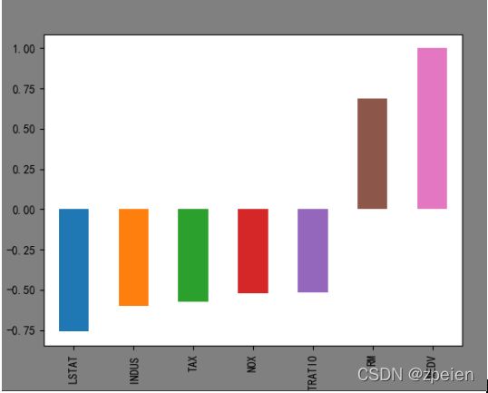
# 计算每一个特征和房价的相关系数
boston_df.corr()['MEDV']

# 各个特征和价格都有明显的线性关系。
plt.figure(facecolor='gray')
corr = boston_df.corr()
corr = corr['MEDV']
corr[abs(corr) > 0.5].sort_values().plot.bar()

boston_df = boston_df[["CRIM", "INDUS", "RM", "AGE", "RAD", "PTRATIO", "LSTAT", 'MEDV']]
# 目标值
y = np.array(boston_df['MEDV'])
boston_df = boston_df.drop(['MEDV'], axis=1)
# 特征值
X = np.array(boston_df)

from sklearn.model_selection import train_test_split

X_train, X_test, y_train, y_test = train_test_split(X, y, test_size=0.3)


from sklearn import preprocessing

# 初始化标准化器
min_max_scaler = preprocessing.MinMaxScaler()
# 分别对训练和测试数据的特征以及目标值进行标准化处理
X_train = min_max_scaler.fit_transform(X_train)
y_train = min_max_scaler.fit_transform(y_train.reshape(-1, 1))  # reshape(-1,1)指将它转化为1列，行自动确定
X_test = min_max_scaler.fit_transform(X_test)
y_test = min_max_scaler.fit_transform(y_test.reshape(-1, 1))

from sklearn.linear_model import LinearRegression

lr = LinearRegression()
# 使用训练数据进行参数估计
lr.fit(X_train, y_train)
# 使用测试数据进行回归预测
y_test_pred = lr.predict(X_test)


# 使用r2_score对模型评估
from sklearn.metrics import mean_squared_error, mean_absolute_error, r2_score


# 绘图函数
def figure(title, *datalist):
    plt.figure(facecolor='gray', figsize=[16, 8])
    for v in datalist:
        plt.plot(v[0], '-', label=v[1], linewidth=2)
        plt.plot(v[0], 'o')
    plt.grid()
    plt.title(title, fontsize=20)
    plt.legend(fontsize=16)
    plt.show()


# 训练数据的预测值
y_train_pred = lr.predict(X_train)

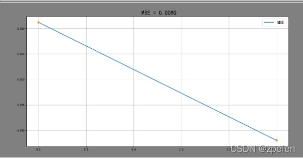
# 计算均分方差
train_MSE = [mean_squared_error(y_train, [np.mean(y_train)] * len(y_train)),
             mean_squared_error(y_train, y_train_pred)]

# 计算平均绝对误差
train_MAE = [mean_absolute_error(y_train, [np.mean(y_train)] * len(y_train)),
             mean_absolute_error(y_train, y_train_pred)]

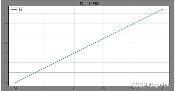
# 计算R2分数
train_R2 = [r2_score(y_train, [np.mean(y_train)] * len(y_train)),
             r2_score(y_train, y_train_pred)]

# 绘制误差图
figure(' MSE = %.4f' % (train_MSE[-1]), [train_MSE, 'MSE'])
figure(' MAE = %.4f' % (train_MAE[-1]), [train_MAE, 'MAE'])
figure(' R2 = %.4f' % (train_R2[-1]), [train_R2, 'R2'])

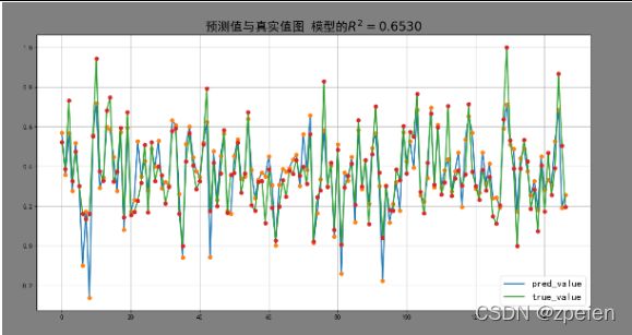
# 绘制预测值与真实值图
figure('预测值与真实值图 模型的' + r'$R^2=%.4f$' % (r2_score(y_train_pred, y_train)), [y_test_pred, 'pred_value'],
       [y_test, 'true_value'])
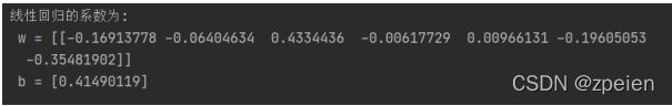
# 线性回归的系数
print('线性回归的系数为:\n w = %s \n b = %s' % (lr.coef_, lr.intercept_))

实验结果：