吴恩达机器学习 逻辑回归 作业2（Python实现）

题目

        在本部分的练习中，您将使用正则化的Logistic回归模型来预测一个制造工厂的微芯片是否通过质量保证（QA），在QA过程中，每个芯片都会经过各种测试来保证它可以正常运行。假设你是这个工厂的产品经理，你拥有一些芯片在两个不同测试下的测试结果，从这两个测试，你希望确定这些芯片是被接受还是拒绝，为了帮助你做这个决定，你有一些以前芯片的测试结果数据集，从中你可以建一个Logistic回归模型。

---

目录

1 正则化逻辑回归函数

2 思路

3 完整代码

---

1 正则化逻辑回归函数

        正则化逻辑回归中，代价函数和梯度函数均有所改变：

2 思路

        注：这部分简述了我的思考过程，代码有不完善之处，也存在部分重复，相比完整版代码有所增删。

        首先读入数据，画出散点图以确定使用曲线阶数。

path=' '  #文件路径
data=pd.read_csv(path,delimiter=',',names=['test1','test2','result'])

'''绘制散点图的函数'''
def plot_data(data):
    pos_data=data[data.result==1]
    neg_data=data[data.result==0]
    plt.scatter(pos_data.test1,pos_data.test2,c='r',marker='+',label='rejected')
    plt.scatter(neg_data.test1,neg_data.test2,c='g',marker='o',label='accepted')
    plt.xlabel('test1')
    plt.ylabel('test2')

plt.figure('raw data')
plot_data(data)
plt.show()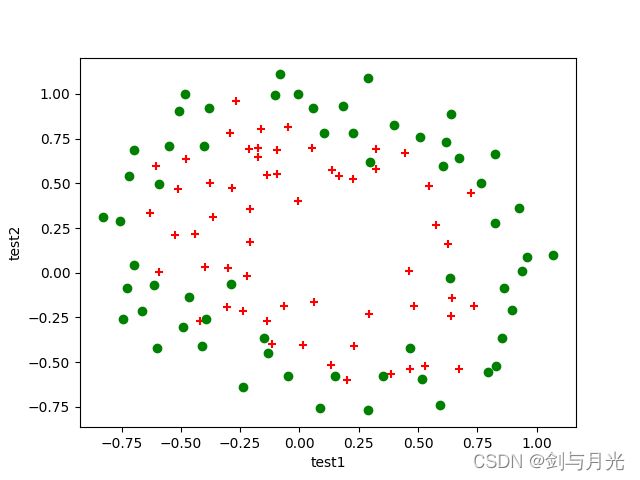

        发现数据点分布杂乱，因此需要进行特征映射以使用高阶曲线。本文后续将采用6阶曲线进行分类。先写出特征映射函数及其对应的求值函数：

def map_feature(x,y,power):
    result=pd.DataFrame(np.ones(x.size),columns=['bias'])
    for i in range(1,power+1):
        for j in range(i+1):
            temp=x**j*y**(i-j)
            result=pd.concat([result,temp],axis=1)
    return result

def feature_cal(x1,x2,power,theta):
    res=0
    pr=0
    for i in range(power+1):
        for j in range(i+1):
            res+=x1**j*x2**(i-j)*theta[pr]
            pr+=1
    return res

        然后根据公式，实现逻辑回归需要使用的三个主要函数：

def sigmoid(x):
    return 1/(1+np.exp(-x))

def cost_function1(theta,x,y):
    size=y.size
    return -1/size*([email protected](sigmoid(x@theta))+(1-y)@np.log(1-sigmoid(x@theta)))

def cost_function2(theta,x,y,lbd=1):
    size=y.size
    theta_p=theta[1:]
    return cost_function1(theta,x,y)+lbd/(2*size)*np.sum(theta_p*theta_p)

def gradient1(theta,x,y):
    size=y.size
    return 1/size*(sigmoid(x@theta)-y).T@x


def gradient2(theta,x,y,lbd=1):
    theta_p=theta/y.size
    theta_p[0]=0
    return gradient1(theta,x,y)+theta_p

        然后就可以处理数值以求解data。求解极值时调用了scipy.optimize库提供的拟牛顿迭代算法bfgs&l_bfgs:

path='D:\机器学习\dataset\ex2data2.txt'
data=pd.read_csv(path,delimiter=',',names=['test1','test2','result'])

x1=data['test1']
x2=data['test2']
x=map_feature(x1,x2,6)
y=data['result']
x=x.values
y=y.values
theta=np.zeros(x.shape[1])

'''任选迭代方法'''
# theta1=opt.fmin_bfgs(f=cost_function2,fprime=gradient2,x0=theta,args=(x,y),maxiter=400)
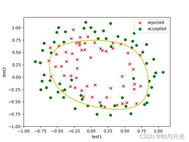
theta1,cost,*u=opt.fmin_l_bfgs_b(func=cost_function2,fprime=gradient2,x0=theta,args=(x,y),maxiter=400)

        最后使用plt.contour方法画出决策边界：

x_axis=np.linspace(-1,1,100)
y_axis=np.linspace(-1,1,100)
zz=np.zeros((x_axis.size,y_axis.size))

for xs in range(x_axis.size):
    for ys in range(y_axis.size):
        zz[xs,ys]=feature_cal(x_axis[xs],y_axis[ys],6,theta1)
plt.figure('boundary')
plot_data(data)
plt.contour(x_axis,y_axis,zz,0,colors='y')

# a=float(input())
# b=float(input())
# c=feature_cal(a,b,6,theta1)
# print(c)
# if c>0:
#     plt.scatter(a,b,c='r',marker='2')
# else:
#     plt.scatter(a,b,c='y',marker='1')

plt.show()

        最后需要对拟合结果进行评估，进行学习率的调整。最后发现学习率 就是不错的状态。

3 完整代码

import numpy as np
import pandas as pd
import matplotlib.pyplot as plt
import scipy.optimize as opt

'''根据data画散点图'''
def plot_data(data):
    pos_data=data[data.result==1]
    neg_data=data[data.result==0]
    plt.scatter(pos_data.test1,pos_data.test2,c='r',marker='x',label='rejected')
    plt.scatter(neg_data.test1,neg_data.test2,c='g',marker='o',label='accepted')
    plt.xlabel('test1')
    plt.ylabel('test2')

'''特征映射'''
def map_feature(x,y,power):
    result=pd.DataFrame(np.ones(x.size),columns=['bias'])
    for i in range(1,power+1):
        for j in range(i+1):
            temp=x**j*y**(i-j)
            result=pd.concat([result,temp],axis=1)
    return result

'''计算特征映射后假设函数的值'''
def feature_cal(x1,x2,power,theta):
    res=0
    pr=0
    for i in range(power+1):
        for j in range(i+1):
            res+=x1**j*x2**(i-j)*theta[pr]
            pr+=1
    return res

'''激活函数'''
def sigmoid(x):
    return 1/(1+np.exp(-x))

'''原始代价函数'''
def cost_function1(theta,x,y):
    size=y.size
    return -1/size*([email protected](sigmoid(x@theta))+(1-y)@np.log(1-sigmoid(x@theta)))

'''正则化代价函数'''
def cost_function2(theta,x,y,lbd=1):
    size=y.size
    theta_p=theta[1:]
    return cost_function1(theta,x,y)+lbd/(2*size)*np.sum(theta_p*theta_p)

'''原始梯度'''
def gradient1(theta,x,y):
    size=y.size
    return 1/size*(sigmoid(x@theta)-y).T@x

'''正则化梯度'''
def gradient2(theta,x,y,lbd=1):
    theta_p=lbd*theta/y.size
    theta_p[0]=0
    return gradient1(theta,x,y)+theta_p


path='D:\机器学习\dataset\ex2data2.txt'
data=pd.read_csv(path,delimiter=',',names=['test1','test2','result'])

# plt.figure('raw data')
# plot_data(data)
# plt.legend()
# plt.show()

x1=data['test1']
x2=data['test2']
x=map_feature(x1,x2,6)
y=data['result']
x=x.values  #将dataFrame转为ndarray
y=y.values
theta=np.zeros(x.shape[1])  
lbd=1 #学习率，可调整

'''选用合适的方式梯度下降'''
# theta1=opt.fmin_bfgs(f=cost_function2,fprime=gradient2,x0=theta,args=(x,y),maxiter=400)
theta1,cost,*u=opt.fmin_l_bfgs_b(func=cost_function2,fprime=gradient2,x0=theta,args=(x,y,lbd),maxiter=400)

'''画出决策边界'''
x_axis=np.linspace(-1,1,100)
y_axis=np.linspace(-1,1,100)
zz=np.zeros((x_axis.size,y_axis.size))
for xs in range(x_axis.size):
    for ys in range(y_axis.size):
        zz[xs,ys]=feature_cal(x_axis[xs],y_axis[ys],6,theta1)
plt.figure('decision_boundary')
plot_data(data)
plt.contour(x_axis,y_axis,zz,0,colors='y',label='boundary')  #函数值为0代表决策边界
plt.legend()
plt.show()

'''输出查准率'''
cnt=0
for i in range(x1.size):
    val=feature_cal(x1[i],x2[i],6,theta1)
    if (val>=0 and y[i]==1) or (val<=0 and y[i]==0):
        cnt+=1
print('查准率: ',cnt/x1.size)