【深度学习】BP神经网络（Backpropagation）简单推导及代码实现

一、原理

1 概括

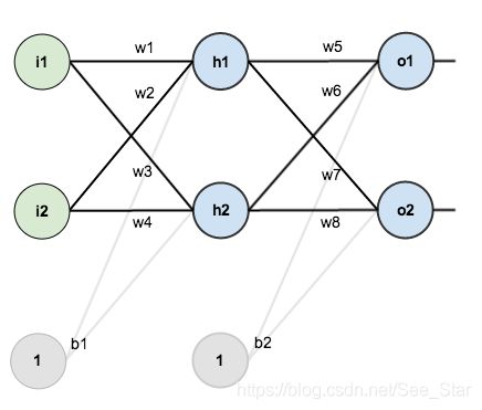
构造一个神经网络含有两个输入，两个隐含层神经元，两个输出神经元。隐藏层和输出元包括权重和偏置。其结构如下：

设置输入和输出数据$(x_i,y_i)$为$(0.05,0.01)$和$(0.1,0.99)$，并为神经元初始化参数，包括权重和偏置。

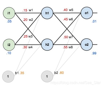
BP神经网络的目标是优化权重，使神经网络学会如何正确地将任意输入映射到输出。以输入0.05和0.1，输出0.01和0.99为训练集进行测试。

2 前项传播

将输入层的0.05和0.10输入到隐藏层，通过初始化的权重和偏差进行计算可得到隐含层的输出。之后通过激活函数对隐含层的输出进行非线性化处理，激活函数使用Sigmoid。
$$f(x)=\frac{1}{1+e^{-x}}$$
计算$h_1$过程如下：
$$\begin{array}{l}ne{t}_{h1}=w_1\ast i_1+w_2\ast i_2+b_1\ast 1\\ \\ ne{t}_{h1}=0.15\ast 0.05+0.2\ast 0.1+0.35\ast 1=0.3775\end{array}$$
非线性化处理，经过sigmoid激活函数后得：
$${\text{ out }}_{h1}=\frac{1}{1+e^{-ne{t}_{h1}}}=\frac{1}{1+e^{-0.3775}}=0.593269992$$
采用相同的方式计算$h_2$得：
$${\text{ out }}_{h2}=0.596884378$$
重复上述过程，利用隐含层的输出计算输出层神经元，下面是$o_1$的计算过程：
$${\text{ net}}_{o1}=w_5\ast {\text{ out }}_{h1}+w_6\ast {\text{ out }}_{h2}+b_2\ast 1$$

$${\text{ net}}_{o1}=0.4\ast 0.593269992+0.45\ast 0.596884378+0.6\ast 1=1.105905967$$

$${\text{ out}}_{o1}=\frac{1}{1+e^{-ne{t}_{o1}}}=\frac{1}{1+e^{-1.105905967}}=0.75136507$$
使用同样的方法计算出$o_2$：
$${\text{out}}_{o2}=0.772928465$$

3 计算误差

使用均方误差（MSE）函数计算神经元的误差，即使用均方误差作为损失函数。
$$MSE(y,y^{\prime })=\frac{{\sum }_{i=1}^n(y_i-y_i^{\prime }{)}^2}{n}$$
其中，$y_i$为第 i 个数据的正确答案，$y_i^{\prime }$为神经网络给出的预测值。在此问题中，$o_1$的期望输出为0.01，但神经网络的真是输出为0.75136507，因此误差为：
$$E_{o1}=\frac{1}{2}{\left({\text{ target }}_{o1}-ou{t}_{o1}\right)}^2=\frac{1}{2}(0.01-0.75136507{)}^2=0.274811083$$
同理得：
$$E_{o2}=0.023560026$$
神经网络的总误差为这些神经元的误差和，即为：
$$E_{\text{total }}=E_{o1}+E_{o2}=0.274811083+0.023560026=0.298371109$$

4 反向传播

使用BP神经网络的目标是更新网络中的每个神经元的权重和偏置，以使它们得实际输出更接近目标输出，从而最大限度地减少每个输出神经元的错误。

4.1 输出层

对于$w_5$，需要知道$w_5$的变化量对于总误差变化量的影响，可表示为$\frac{\partial E_{\text{total }}}{\partial w_5}$，即$w_5$的梯度。

通过链式法则可得：
$$\frac{\partial E_{\text{total }}}{\partial w_5}=\frac{\partial E_{\text{total }}}{\partial {\text{ out }}_{o1}}\ast \frac{\partial {\text{ out }}_{o1}}{\partial {\text{ net }}_{o1}}\ast \frac{\partial {\text{ net }}_{o1}}{\partial w_5}$$

这是可视化过程：

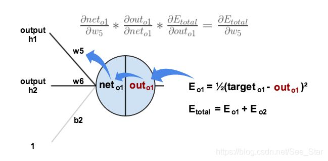
我们需要解决方程的每一个步骤。

首先要分析输出对总误差的影响：
$$E_{\text{total }}=\frac{1}{2}{\left({\text{ target}}_{o1}-{\text{ out }}_{o1}\right)}^2+\frac{1}{2}{\left({\mathrm{target}}_{o2}-{\text{ out}}_{o2}\right)}^2$$
$$\frac{\partial E_{\text{total }}}{\partial ou{t}_{o1}}=2\ast \frac{1}{2}{\left({\text{ target}}_{o1}-ou{t}_{o1}\right)}^{2-1}\ast -1+0$$
$$\frac{\partial E_{\text{totol }}}{\partial ou{t}_{o1}}=-\left({\text{ target}}_{o1}-ou{t}_{o1}\right)=-(0.01-0.75136507)=0.74136507$$

对激活函数求偏导得：
$${\text{ out }}_{o1}=\frac{1}{1+e^{-{\text{net }}_{o1}}}$$
$$\frac{\partial {\text{ out}}_{o1}}{\partial {\text{ net}}_{o1}}={\text{ out}}_{o1}\left(1-{\text{ out}}_{o1}\right)=0.75136507(1-0.75136507)=0.186815602$$

最后，计算$ne{t}_{o1}$对$w_5$的偏导：
$${net}_{o1}=w_5\ast {out}_{h1}+w_6\ast {\text{ out }}_{h2}+b_2\ast 1$$
$$\frac{\partial {net}_{o1}}{\partial w_5}=1\ast {out}_{h1}\ast w_5^{(1-1)}+0+0={out}_{h1}=0.593269992$$
把以上的计算结果乘到一起得：
$$\frac{\partial E_{tatal}}{\partial w_5}=\frac{\partial E_{total}}{\partial {out}_{o1}}\ast \frac{\partial {out}_{o1}}{\partial ne{t}_{o1}}\ast \frac{\partial ne{t}_{a1}}{\partial w_5}$$
$$\frac{\partial E_{total}}{\partial w_5}=0.74136507\ast 0.186815602\ast 0.593269992=0.082167041$$
为了减少误差，我们对权重进行修正，即用当前的权重中减去修正值乘以学习率，此处设置学习率为0.5：
$$w_5^{+}=w_5-\eta \ast \frac{\partial E_{total}}{\partial w_5}=0.4-0.5\ast 0.082167041=0.35891648$$
重复以上步骤可计算出$w_6$、$w_7$和$w_8$：
$$\begin{array}{l}{w}_6^{+}=0.408666186\\ w_7^{+}=0.511301270\\ w_8^{+}=0.561370121\end{array}$$
此时已经计算出输出层的新权重，当计算出隐含层的权重后，对整个网络的权重进行更新，下面计算隐含层的权重。

4.2 隐含层

接下来，继续使用反向传播计算$w_1$、$w_2$、$w_3$和$w_4$。根据链式法则可得：
$$\frac{\partial E_{total}}{\partial w_1}=\frac{\partial E_{total}}{\partial ou{t}_{h1}}\ast \frac{\partial ou{t}_{h1}}{\partial ne{t}_{h1}}\ast \frac{\partial ne{t}_{h1}}{\partial w_1}$$
可视化图像为：

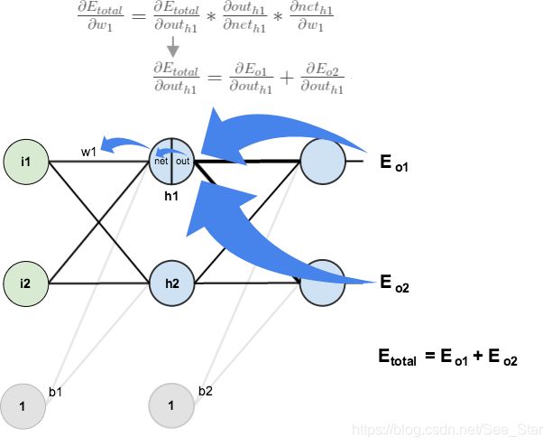
接下来将采用相似的方式处理隐含层的神经元，但是略有不同，考虑到每个隐含层的神经元的输出连接到多个输出，$ou{t}_{h1}$影响$ou{t}_{o1}$和$ou{t}_{o2}$，因此计算$\frac{\partial E_{\text{total }}}{{dout}_{h1}}$需考虑所有输出神经元：
$$\frac{\partial E_{total}}{\partial ou{t}_{h1}}=\frac{\partial E_{o1}}{\partial ou{t}_{h1}}+\frac{\partial E_{a2}}{\partial ou{t}_{h1}}$$
其中，
$$\frac{\partial E_{o1}}{\partial ou{t}_{h1}}=\frac{\partial E_{o1}}{\partial ne{t}_{o1}}\ast \frac{\partial ne{t}_{o1}}{\partial ou{t}_{h1}}$$
可通过之前的结果计算$\frac{\partial E_{o1}}{\partial {net}_{o1}}$：
$$\frac{\partial E_{a1}}{\partial ne{t}_{o1}}=\frac{\partial E_{o1}}{\partial ou{t}_{o1}}\ast \frac{\partial {\text{ out }}_{t_0}}{\partial ne{t}_{o1}}=0.74136507\ast 0.186815602=0.138498562$$
并且，$\frac{\partial {net}_{o1}}{\partial {out}_{h1}}=w_5$：
$${net}_{o1}=w_5\ast ou{t}_{h1}+w_6\ast ou{t}_{h2}+b_2\ast 1$$
$$\frac{\partial ne{t}_{o1}}{\partial ou{t}_{h1}}=w_5=0.40$$
将其乘起来得：
$$\frac{\partial E_{o1}}{\partial ou{t}_{h1}}=\frac{\partial E_{o1}}{\partial ne{t}_{o1}}\ast \frac{\partial ne{t}_{o1}}{\partial ou{t}_{h1}}=0.138498562\ast 0.40=0.055399425$$
同理可得，
$$\frac{\partial E_{o2}}{\partial ou{t}_{h1}}=-0.019049119$$
因此，
$$\frac{\partial E_{total}}{\partial ou{t}_{h1}}=\frac{\partial E_{o1}}{\partial ou{t}_{h1}}+\frac{\partial E_{o2}}{\partial ou{t}_{h1}}=0.055399425+-0.019049119=0.036350306$$
现在知道$\frac{\partial E_{total}}{\partial ou{t}_{h1}}$，需要计算出$\frac{\partial ou{t}_{h1}}{\partial ne{t}_{h1}}$和$\frac{\partial ne{t}_{h1}}{\partial w}$：
$$ou{t}_{h1}=\frac{1}{1+e^{-ne{t}_{h1}}}$$
$$\frac{\partial ou{t}_{h1}}{\partial ne{t}_{h1}}=ou{t}_{h1}\left(1-ou{t}_{h1}\right)=0.59326999(1-0.59326999)=0.241300709$$
采用相同的方式计算网络输入$h_1$对$w$的偏导数：
$$ne{t}_{h1}=w_1\ast i_1+w_3\ast i_2+b_1\ast 1$$
$$\frac{\partial ne{t}_{h1}}{\partial w_1}=i_1=0.05$$
把它们乘到一起：
$$\frac{\partial E_{total}}{\partial w_1}=\frac{\partial E_{totat}}{\partial ou{t}_{h1}}\ast \frac{\partial ou{t}_{h1}}{\partial ne{t}_{h1}}\ast \frac{\partial ne{t}_{h1}}{\partial w_1}$$
$$\frac{\partial E_{total}}{\partial w_1}=0.036350306\ast 0.241300709\ast 0.05=0.000438568$$
现在，可以对$w_1$进行更新：
$$w_1^{+}=w_1-\eta \ast \frac{\partial E_{total}}{\partial w_1}=0.15-0.5\ast 0.000438568=0.149780716$$
重复以上步骤计算$w_2$、$w_3$和$w_4$：
$$\begin{array}{l}{w}_2^{+}=0.19956143\\ w_3^{+}=0.24975114\\ w_4^{+}=0.29950229\end{array}$$
最后，更新所有神经元的权重，当输入$0.05$和$0.1$时，网络上的总误差从为$0.298371109$转变为$0.291027924$。 重复以上过程$10,000$次后，总误差将降到$3.5102\ast 10^{-5}$。 此时，当输入$0.05$和$0.1$时，两个输出神经元输出的结果分别为$0.015912196$（期望值为$0.01$）和$0.984065734$（期望值为$0.99$）。训练$20,000$次后，总误差将降到$7.837\ast 10^{-6}$。

二、代码

import random
import math

#
# Shorthand:
#   "pd_" as a variable prefix means "partial derivative"
#   "d_" as a variable prefix means "derivative"
#   "_wrt_" is shorthand for "with respect to"
#   "w_ho" and "w_ih" are the index of weights from hidden to output layer neurons and input to hidden layer neurons respectively
#
# Comment references:
#
# [1] Wikipedia article on Backpropagation
#   http://en.wikipedia.org/wiki/Backpropagation#Finding_the_derivative_of_the_error
# [2] Neural Networks for Machine Learning course on Coursera by Geoffrey Hinton
#   https://class.coursera.org/neuralnets-2012-001/lecture/39
# [3] The Back Propagation Algorithm
#   https://www4.rgu.ac.uk/files/chapter3%20-%20bp.pdf

class NeuralNetwork:
    LEARNING_RATE = 0.5

    def __init__(self, num_inputs, num_hidden, num_outputs, hidden_layer_weights = None, hidden_layer_bias = None, output_layer_weights = None, output_layer_bias = None):
        self.num_inputs = num_inputs

        self.hidden_layer = NeuronLayer(num_hidden, hidden_layer_bias)
        self.output_layer = NeuronLayer(num_outputs, output_layer_bias)

        self.init_weights_from_inputs_to_hidden_layer_neurons(hidden_layer_weights)
        self.init_weights_from_hidden_layer_neurons_to_output_layer_neurons(output_layer_weights)

    def init_weights_from_inputs_to_hidden_layer_neurons(self, hidden_layer_weights):
        weight_num = 0
        for h in range(len(self.hidden_layer.neurons)):
            for i in range(self.num_inputs):
                if not hidden_layer_weights:
                    self.hidden_layer.neurons[h].weights.append(random.random())
                else:
                    self.hidden_layer.neurons[h].weights.append(hidden_layer_weights[weight_num])
                weight_num += 1

    def init_weights_from_hidden_layer_neurons_to_output_layer_neurons(self, output_layer_weights):
        weight_num = 0
        for o in range(len(self.output_layer.neurons)):
            for h in range(len(self.hidden_layer.neurons)):
                if not output_layer_weights:
                    self.output_layer.neurons[o].weights.append(random.random())
                else:
                    self.output_layer.neurons[o].weights.append(output_layer_weights[weight_num])
                weight_num += 1

    def inspect(self):
        print('------')
        print('* Inputs: {}'.format(self.num_inputs))
        print('------')
        print('Hidden Layer')
        self.hidden_layer.inspect()
        print('------')
        print('* Output Layer')
        self.output_layer.inspect()
        print('------')

    def feed_forward(self, inputs):
        hidden_layer_outputs = self.hidden_layer.feed_forward(inputs)
        return self.output_layer.feed_forward(hidden_layer_outputs)

    # Uses online learning, ie updating the weights after each training case
    def train(self, training_inputs, training_outputs):
        self.feed_forward(training_inputs)

        # 1. Output neuron deltas
        pd_errors_wrt_output_neuron_total_net_input = [0] * len(self.output_layer.neurons)
        for o in range(len(self.output_layer.neurons)):

            # ∂E/∂zⱼ
            pd_errors_wrt_output_neuron_total_net_input[o] = self.output_layer.neurons[o].calculate_pd_error_wrt_total_net_input(training_outputs[o])

        # 2. Hidden neuron deltas
        pd_errors_wrt_hidden_neuron_total_net_input = [0] * len(self.hidden_layer.neurons)
        for h in range(len(self.hidden_layer.neurons)):

            # We need to calculate the derivative of the error with respect to the output of each hidden layer neuron
            # dE/dyⱼ = Σ ∂E/∂zⱼ * ∂z/∂yⱼ = Σ ∂E/∂zⱼ * wᵢⱼ
            d_error_wrt_hidden_neuron_output = 0
            for o in range(len(self.output_layer.neurons)):
                d_error_wrt_hidden_neuron_output += pd_errors_wrt_output_neuron_total_net_input[o] * self.output_layer.neurons[o].weights[h]

            # ∂E/∂zⱼ = dE/dyⱼ * ∂zⱼ/∂
            pd_errors_wrt_hidden_neuron_total_net_input[h] = d_error_wrt_hidden_neuron_output * self.hidden_layer.neurons[h].calculate_pd_total_net_input_wrt_input()

        # 3. Update output neuron weights
        for o in range(len(self.output_layer.neurons)):
            for w_ho in range(len(self.output_layer.neurons[o].weights)):

                # ∂Eⱼ/∂wᵢⱼ = ∂E/∂zⱼ * ∂zⱼ/∂wᵢⱼ
                pd_error_wrt_weight = pd_errors_wrt_output_neuron_total_net_input[o] * self.output_layer.neurons[o].calculate_pd_total_net_input_wrt_weight(w_ho)

                # Δw = α * ∂Eⱼ/∂wᵢ
                self.output_layer.neurons[o].weights[w_ho] -= self.LEARNING_RATE * pd_error_wrt_weight

        # 4. Update hidden neuron weights
        for h in range(len(self.hidden_layer.neurons)):
            for w_ih in range(len(self.hidden_layer.neurons[h].weights)):

                # ∂Eⱼ/∂wᵢ = ∂E/∂zⱼ * ∂zⱼ/∂wᵢ
                pd_error_wrt_weight = pd_errors_wrt_hidden_neuron_total_net_input[h] * self.hidden_layer.neurons[h].calculate_pd_total_net_input_wrt_weight(w_ih)

                # Δw = α * ∂Eⱼ/∂wᵢ
                self.hidden_layer.neurons[h].weights[w_ih] -= self.LEARNING_RATE * pd_error_wrt_weight

    def calculate_total_error(self, training_sets):
        total_error = 0
        for t in range(len(training_sets)):
            training_inputs, training_outputs = training_sets[t]
            self.feed_forward(training_inputs)
            for o in range(len(training_outputs)):
                total_error += self.output_layer.neurons[o].calculate_error(training_outputs[o])
        return total_error

class NeuronLayer:
    def __init__(self, num_neurons, bias):

        # Every neuron in a layer shares the same bias
        self.bias = bias if bias else random.random()

        self.neurons = []
        for i in range(num_neurons):
            self.neurons.append(Neuron(self.bias))

    def inspect(self):
        print('Neurons:', len(self.neurons))
        for n in range(len(self.neurons)):
            print(' Neuron', n)
            for w in range(len(self.neurons[n].weights)):
                print('  Weight:', self.neurons[n].weights[w])
            print('  Bias:', self.bias)

    def feed_forward(self, inputs):
        outputs = []
        for neuron in self.neurons:
            outputs.append(neuron.calculate_output(inputs))
        return outputs

    def get_outputs(self):
        outputs = []
        for neuron in self.neurons:
            outputs.append(neuron.output)
        return outputs

class Neuron:
    def __init__(self, bias):
        self.bias = bias
        self.weights = []

    def calculate_output(self, inputs):
        self.inputs = inputs
        self.output = self.squash(self.calculate_total_net_input())
        return self.output

    def calculate_total_net_input(self):
        total = 0
        for i in range(len(self.inputs)):
            total += self.inputs[i] * self.weights[i]
        return total + self.bias

    # Apply the logistic function to squash the output of the neuron
    # The result is sometimes referred to as 'net' [2] or 'net' [1]
    def squash(self, total_net_input):
        return 1 / (1 + math.exp(-total_net_input))

    # Determine how much the neuron's total input has to change to move closer to the expected output
    #
    # Now that we have the partial derivative of the error with respect to the output (∂E/∂yⱼ) and
    # the derivative of the output with respect to the total net input (dyⱼ/dzⱼ) we can calculate
    # the partial derivative of the error with respect to the total net input.
    # This value is also known as the delta (δ) [1]
    # δ = ∂E/∂zⱼ = ∂E/∂yⱼ * dyⱼ/dzⱼ
    #
    def calculate_pd_error_wrt_total_net_input(self, target_output):
        return self.calculate_pd_error_wrt_output(target_output) * self.calculate_pd_total_net_input_wrt_input();

    # The error for each neuron is calculated by the Mean Square Error method:
    def calculate_error(self, target_output):
        return 0.5 * (target_output - self.output) ** 2

    # The partial derivate of the error with respect to actual output then is calculated by:
    # = 2 * 0.5 * (target output - actual output) ^ (2 - 1) * -1
    # = -(target output - actual output)
    #
    # The Wikipedia article on backpropagation [1] simplifies to the following, but most other learning material does not [2]
    # = actual output - target output
    #
    # Alternative, you can use (target - output), but then need to add it during backpropagation [3]
    #
    # Note that the actual output of the output neuron is often written as yⱼ and target output as tⱼ so:
    # = ∂E/∂yⱼ = -(tⱼ - yⱼ)
    def calculate_pd_error_wrt_output(self, target_output):
        return -(target_output - self.output)

    # The total net input into the neuron is squashed using logistic function to calculate the neuron's output:
    # yⱼ = φ = 1 / (1 + e^(-zⱼ))
    # Note that where ⱼ represents the output of the neurons in whatever layer we're looking at and ᵢ represents the layer below it
    #
    # The derivative (not partial derivative since there is only one variable) of the output then is:
    # dyⱼ/dzⱼ = yⱼ * (1 - yⱼ)
    def calculate_pd_total_net_input_wrt_input(self):
        return self.output * (1 - self.output)

    # The total net input is the weighted sum of all the inputs to the neuron and their respective weights:
    # = zⱼ = netⱼ = x₁w₁ + x₂w₂ ...
    #
    # The partial derivative of the total net input with respective to a given weight (with everything else held constant) then is:
    # = ∂zⱼ/∂wᵢ = some constant + 1 * xᵢw₁^(1-0) + some constant ... = xᵢ
    def calculate_pd_total_net_input_wrt_weight(self, index):
        return self.inputs[index]

###

# Blog post example:

nn = NeuralNetwork(2, 2, 2, hidden_layer_weights=[0.15, 0.2, 0.25, 0.3], hidden_layer_bias=0.35, output_layer_weights=[0.4, 0.45, 0.5, 0.55], output_layer_bias=0.6)
for i in range(10000):
    nn.train([0.05, 0.1], [0.01, 0.99])
    print(f"epoch:{i}\terror:{round(nn.calculate_total_error([[[0.05, 0.1], [0.01, 0.99]]]), 9)}")

# XOR example:

# training_sets = [
#     [[0, 0], [0]],
#     [[0, 1], [1]],
#     [[1, 0], [1]],
#     [[1, 1], [0]]
# ]

# nn = NeuralNetwork(len(training_sets[0][0]), 5, len(training_sets[0][1]))
# for i in range(10000):
#     training_inputs, training_outputs = random.choice(training_sets)
#     nn.train(training_inputs, training_outputs)
#     print(i, nn.calculate_total_error(training_sets))

参考：https://mattmazur.com/2015/03/17/a-step-by-step-backpropagation-example/