【图像处理】PyTorch实战之CIFAR10数据集分类（LeNet分类器）

首先这是一个官方demo，PyTorch官网入门实现一个图像分类器
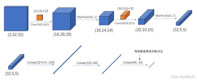
下图是卷积，池化，全连接层在神经网络中的作用（分工）

本文是学习B站深度学习与图像处理的up做的笔记
本文参考主要如下：
1.B站宝藏up讲解视频
2.PyTorch官方文档
3.某博主的课程笔记

官方demo的流程

1. model.py：定义LeNet网络模型
2. train.py：加载数据集并训练，训练集计算loss，测试集计算accuracy，保存训练好的网络参数
3. predict.py：得到训练好的网络参数后，用自己找的图像进行分类测试

model.py代码

import torch.nn as nn
import torch.nn.functional as F


class LeNet(nn.Module):
    def __init__(self):    # 初始化函数
        super(LeNet, self).__init__() # 涉及到多继承一般会使用super函数
        """
        卷积层的计算公式
        N = (W - F + 2P) / S + 1
        1.输入的图片大小为 w*w
        2.Filter大小F*F
        3.步长S
        4.padding的像素数p
        """
        # 第一个参数代表输入特征矩阵的参数 第二个函数是输入卷积层的个数 第三个参数代表卷积层的大小
        self.conv1 = nn.Conv2d(3, 16, 5)
        # 第一个参数是池化和的大小 第二个参数为步距
        self.pool1 = nn.MaxPool2d(2, 2)
        self.conv2 = nn.Conv2d(16, 32, 5)
        self.pool2 = nn.MaxPool2d(2, 2)
        self.fc1 = nn.Linear(32*5*5, 120)
        self.fc2 = nn.Linear(120, 84)
        self.fc3 = nn.Linear(84, 10)

    def forward(self, x):            # 定义正向传播
        x = F.relu(self.conv1(x))    # input(3, 32, 32) output(16, 28, 28)
        x = self.pool1(x)            # output(16, 14, 14)
        # relu为激活函数
        x = F.relu(self.conv2(x))    # output(32, 10, 10)
        x = self.pool2(x)            # output(32, 5, 5)
        # view函数的作用是吧特征矩阵展开为一维向量形式
        # 这里的-1不是一个有意义的数，在这“暂时占位”，可以把它理解为未知数x，他会根据第二个维度反推这个x
        x = x.view(-1, 32*5*5)       # output(32*5*5)
        x = F.relu(self.fc1(x))      # output(120)
        x = F.relu(self.fc2(x))      # output(84)
        x = self.fc3(x)              # output(10)
        return x

Conv2d

PyTorch中Tensor通道的排列顺序是[batch, channel, height, width]
我们通常常用的卷积（Conv2d）在pytorch中对应的函数是：

torch.nn.Conv2d(in_channels, 
                out_channels, 
                kernel_size, 
                stride=1, 
                padding=0, 
                dilation=1, 
                groups=1, 
                bias=True, 
                padding_mode='zeros')

• in_channels参数：代表输入特征矩阵的深度，一张RGB彩色图像为3
• out_channels参数：代表卷积核的个数
• kernel_size参数：代表卷积核的尺寸，输入可以是int类型，也可以是tuple（height，width）类型
• stride参数：代表卷积核的步距默认为1，同样可以是int或者tuple类型
• padding参数：代表在输入特征矩阵四周补零的情况默认为0，同样的输入可以为int型，如1代表上下左右方向各补一圈0，如果输入为tuple（2，1）代表在上方补两行，下方补两行，左边补一列，右边补一列。如果需要实现更灵活的padding方式，可以使用nn.ZeroPad2d方法
• bias参数：表示是否使用偏置（默认使用）
• dilation，group是高阶用法，很少用到

代码中卷积层计算公式： N = (W - F + 2P) / S + 1
有的时候N会为非整数的情况，此时在卷积过程中会直接将最后一行以及最后一列给忽略掉，以保证N为整数

train.py代码

import numpy as np
import torch
import torchvision
import torch.nn as nn
from matplotlib import pyplot as plt

from model import LeNet
import torch.optim as optim
import torchvision.transforms as transforms

transform = transforms.Compose(
    [transforms.ToTensor(),
     transforms.Normalize((0.5, 0.5, 0.5), (0.5, 0.5, 0.5))])

# 50000张训练图片
# 第一次使用时要将download设置为True才会自动去下载数据集
train_set = torchvision.datasets.CIFAR10(root='./data', train=True,
                                         download=True, transform=transform)
# 这四个参数分别代表导入的训练集 每批训练的样本数 是否打乱训练集 线程数
train_loader = torch.utils.data.DataLoader(train_set, batch_size=36,
                                           shuffle=True, num_workers=0)

# 10000张验证图片
# 第一次使用时要将download设置为True才会自动去下载数据集
val_set = torchvision.datasets.CIFAR10(root='./data', train=False,
                                       download=False, transform=transform)
val_loader = torch.utils.data.DataLoader(val_set, batch_size=10000,
                                         shuffle=False, num_workers=0)
val_data_iter = iter(val_loader)
val_image, val_label = val_data_iter.next()

classes = ('plane', 'car', 'bird', 'cat',
           'deer', 'dog', 'frog', 'horse', 'ship', 'truck')

# def imshow(img):
#     img = img / 2 + 0.5
#     npimg = img.numpy()  # 将图像反标准化
#     plt.imshow(np.transpose(npimg, (1, 2, 0)))
#     plt.show()
#
# 需要显示图片的话，即把 batch_size=10000中的10000改为4，因为10000太大了，显示不出来
# print(' '.join('%5s' % classes[val_label[j]] for j in range(4)))
# imshow(torchvision.utils.make_grid(val_image))

net = LeNet()  # 实例化
loss_function = nn.CrossEntropyLoss()  # 定义损失函数
optimizer = optim.Adam(net.parameters(), lr=0.001)  # 优化器 第一个参数为需要训练的参数，lr为学习率

# 将训练集迭代五轮
for epoch in range(5):  # loop over the dataset multiple times

    running_loss = 0.0 # 累加训练过程中的损失
    for step, data in enumerate(train_loader, start=0):
        # get the inputs; data is a list of [inputs, labels]
        inputs, labels = data

        # zero the parameter gradients
        """
        为什么每计算一个batch，就需要调用一次optimizer.zero_grad()？
        因为如果不清楚历史梯度，就会对计算的历史梯度进行累加（通过这个特性你能够变相实现一个很大的batch数值的训练
        """
        optimizer.zero_grad() # 将历史损失梯度清零
        # forward + backward + optimize
        outputs = net(inputs)
        loss = loss_function(outputs, labels)
        loss.backward() # 反向传播
        optimizer.step()# 参数更新

        # print statistics
        running_loss += loss.item()
        if step % 500 == 499:  # print every 500 mini-batches
            with torch.no_grad(): # with是一个上下文管理器
                outputs = net(val_image)  # [batch, 10]
                predict_y = torch.max(outputs, dim=1)[1]
                accuracy = torch.eq(predict_y, val_label).sum().item() / val_label.size(0)

                print('[%d, %5d] train_loss: %.3f  test_accuracy: %.3f' %
                      (epoch + 1, step + 1, running_loss / 500, accuracy))
                running_loss = 0.0

print('Finished Training')

save_path = './Lenet.pth'
torch.save(net.state_dict(), save_path)

名词解释
epoch：对训练集的全部数据进行一次完整的训练，也称迭代，称为一次eopch
batch：每批数据大小
iteration或step：对一个batch数据训练的过程称为一个iteration或step

打印结果如下

[1,   500] train_loss: 1.761  test_accuracy: 0.436
[1,  1000] train_loss: 1.463  test_accuracy: 0.504
[2,   500] train_loss: 1.254  test_accuracy: 0.572
[2,  1000] train_loss: 1.184  test_accuracy: 0.587
[3,   500] train_loss: 1.038  test_accuracy: 0.612
[3,  1000] train_loss: 1.044  test_accuracy: 0.628
[4,   500] train_loss: 0.920  test_accuracy: 0.654
[4,  1000] train_loss: 0.920  test_accuracy: 0.652
[5,   500] train_loss: 0.830  test_accuracy: 0.662
[5,  1000] train_loss: 0.855  test_accuracy: 0.666
Finished Training

那么现在我们可以去验证一下，首先从百度上找到一张图片，我找到的是飞机图片，来验证一下

验证代码predict.py

import torch
import torchvision.transforms as transforms
from PIL import Image

from model import LeNet


def main():
    transform = transforms.Compose(
        [transforms.Resize((32, 32)), # 将图片强制转换成32*32的
         transforms.ToTensor(),
         transforms.Normalize((0.5, 0.5, 0.5), (0.5, 0.5, 0.5))])

    classes = ('plane', 'car', 'bird', 'cat',
               'deer', 'dog', 'frog', 'horse', 'ship', 'truck')

    net = LeNet() # 实例化
    net.load_state_dict(torch.load('Lenet.pth')) # 载入权重文件

    im = Image.open('1.png')
    im = transform(im)  # [C, H, W]
    im = torch.unsqueeze(im, dim=0)  # [N, C, H, W]

    with torch.no_grad():
        outputs = net(im)  # 将图像传到网络中
        predict = torch.max(outputs, dim=1)[1].numpy() #dim代表维度
    print(classes[int(predict)])

    with torch.no_grad():
        outputs = net(im)  # 将图像传到网络中
        predict = torch.softmax(outputs,dim=1)
    print(predict)


if __name__ == '__main__':
    main()

先把找到的图片放在目录下


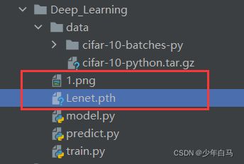
运行代码，查看结果：
同时我们还打印了一下概率，可以看出是飞机的概率最高，高达98%
听说猫和狗的图片容易识别出错

plane
tensor([[9.8213e-01, 3.0834e-06, 4.1951e-04, 1.1767e-06, 3.5559e-04, 8.5063e-07,
         1.6793e-06, 1.6772e-06, 1.7021e-02, 6.4978e-05]])

迷茫就去跑跑步，焦虑就去吃肉肉，难过就去听听歌，委屈就找个没人的地方喊出来，孤独就去花店里买束花。先把五官哄开心了，再去设法营救受困的灵魂。