Image Super-resolution Reconstruction Based on Bionic Intelligence

Image Super-resolution Reconstruction Based on Bionic Intelligence

基于仿生智能的图像超分辨率重建–理解和代码还原

说明：本文是参照20年IEEE上的一篇文章，进行阅读，理解，以及根据自己的理解进行的复现（python），因为版本问题，有些代码可能无法成功运行。我以后还会在此基础上进行改进，现在先把主要内容罗列出来。
文章作者：
Xin Wang, Qiong Wang, Guofang Lv
Jiangsu Key Laboratory of Image and Video Understanding for Social Safety,
Nanjing University of Science and Technology, Nanjing, China
College of Computer and Information, Hohai University, Nanjing, China

内容理解

主要思想：传统的超分辨率重建方法通常将低分辨率图像作为一个整体进行处理，忽略了图像块之间的差异，导致重建效果不佳。
此文章采用斑块的概念，将“斑块”作为超分辨率重构的基本单元。
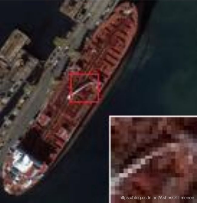
此文章将生物视觉注意机制启发的方法应用于初始重建结果，以检测出显著区域（文章重点）。然后，将超分辨率卷积神经网络模型应用于显著图像块，以获得精确的重建结果

步骤：

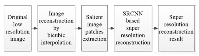
step1：双三次插值图像重建
首先使用双三次插值法重建原始分辨率图像，得到Xinit。
step2：显著图像块提取
2.1用FT技术计算Xinit.
2.2然后自适应阈值运算得到二进制显著映射Winit。
2.3将Xinit分为n个块。基于Winit，如果至少五分之一的图像块是白色的，则将此图像块视为显著性块；否则，将Pk视为不显著的。
step3：基于SRCNN的超分辨率重建
将SRCNN分别应用于每个显著图像块

step1 双三次插值法（bicubic interpolation）

插值方法简单来说就是我们输入一个低分辨率图像，我们得到它每个像素点上的像素值，来对它进行插入，填充近一些空的像素点，通过一定的办法计算出这些空像素点的像素值。

1.此算法涉及到16个像素点，其中P00代表目标插值图中某像素点在原图中最接近的像素点。
（1.1，1.2）——>P00：（1，1）
而最终插值后的图像（x，y）的值为以下16个像素点的权重卷积之和。

2.假设源图像A大小为mn，缩放K倍后的目标图像B的大小为MN，即K=M/m。我们想要求出目标图像B中每一像素点(X,Y)的值，必须先找出像素(X,Y)在源图像A中对应的像素(x,y)，再根据源图像A距离像素(x,y)最近的16个像素点作为计算目标图像B(X,Y)处像素值的参数，利用BiCubic基函数求出16个像素点的权重，图B像素(x,y)的值就等于16个像素点的加权叠加。

3.开始构造BiCubic 函数，可用以下函数近似：

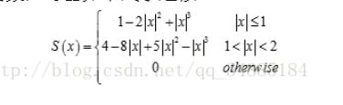
# 产生16个像素点不同的权重
def BiBubic(x):
     x=abs(x)
     if x<=1:
        return 1-2*(x**2)+(x**3)
     elif x<2:
         return 4-8*x+5*(x**2)-(x**3)
     else:
         return 0

4.然后我们要做的就是求出BiCubic函数中的参数x,从而获得上面所说的16个像素所对应的权重W(x)。BiCubic基函数是一维的，而像素是二维的，所以我们将像素点的行与列分开计算。BiCubic函数中的参数x表示该像素点到P点的距离，例如a00距离P(x+u,y+v)的距离为(1+u,1+v)，因此a00的横坐标权重i_0=W(1+u)，纵坐标权重j_0=W(1+v)，a00对B(X,Y)的贡献值为：（a00像素值）* i_0* j_0。因此，a0X的横坐标权重分别为W(1+u)，W(u)，W(1-u)，W(2-u)；ay0的纵坐标权重分别为W(1+v)，W(v)，W(1-v)，W(2-v)；B(X,Y)像素值为

加权算法：

# 双三次插值算法
# dstH为目标图像的高，dstW为目标图像的宽
def BiCubic_interpolation(img,dstH,dstW):  #传入原始图像/目标图像的高/目标图像的宽
     scrH,scrW,_=img.shape					#获取原图像的高度和宽度
     #img=np.pad(img,((1,3),(1,3),(0,0)),'constant')
     retimg=np.zeros((dstH,dstW,3),dtype=np.uint8)
     for i in range(dstH):
         for j in range(dstW):
             scrx=i*(scrH/dstH)
             scry=j*(scrW/dstW)
             x=math.floor(scrx)
             y=math.floor(scry)
             u=scrx-x
             v=scry-y
             tmp=0
             for ii in range(-1,2):
                 for jj in range(-1,2):
                     if x+ii<0 or y+jj<0 or x+ii>=scrH or y+jj>=scrW:
                         continue
                     tmp+=img[x+ii,y+jj]*BiBubic(ii-u)*BiBubic(jj-v)      #产生16个像素点不同的权重
             retimg[i,j]=np.clip(tmp,0,255)
     return retimg

5.得到Xinit

图左是原始的低分辨率图像img。图右是用双三次插值法重建的图像Xinit。可以看出，虽然图像尺寸变大了，但还是有点模糊。

step2：显著图像块提取

2.1用FT技术计算Xinit.

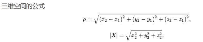
原理：计算Lab空间下每点与均值的欧式距离作为显著值
note1：
Lab是由一个亮度通道（channel）和两个颜色通道组成的。在Lab颜色空间中，每个颜色用L、a、b三个数字表示，各个分量的含义是这样的：
- L代表亮度- a代表从绿色到红色的分量- b代表从蓝色到黄色的分量*
note2：
欧式距离计算

	 **代码**：

def FT(img):
    #img = img[...,::-1]                         #把RGB(或BRG)转换成BGR(或者RGB)。
    img = cv2.cvtColor(img, cv2.COLOR_BGR2RGB)  #将传入的图片转成RGB格式
    img = cv2.GaussianBlur(img,(5,5), 0)        #第一步：高斯滤波
    lab = cv2.cvtColor(img, cv2.COLOR_RGB2LAB)  #第二步：转成LAB色彩空间格式
    l_mean = np.average(lab[0])                 #第三步：计算
    a_mean = np.average(lab[1])
    b_mean = np.average(lab[2])
    inits = np.square(lab - np.array([l_mean, a_mean, b_mean]))
    inits = np.sum(lab,axis=2)
    inits = lab/np.max(lab)
    return inits

2.2自适应阈值运算得到二进制显著映射Winit.
原理：根据图像不同区域亮度分布，计算其局部阈值，所以对于图像不同区域，能够自适应计算不同的阈值，因此被称为自适应阈值法。
代码：

def Adaptive(img):
    GrayImage=cv2.cvtColor(img,cv2.COLOR_BGR2GRAY)
    GrayImage= cv2.medianBlur(GrayImage,5)      # 中值滤波
    Winit = cv2.adaptiveThreshold(GrayImage,255,cv2.ADAPTIVE_THRESH_GAUSSIAN_C,\
                    cv2.THRESH_BINARY,3,5)
    return Winit 

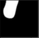
得到Winit：

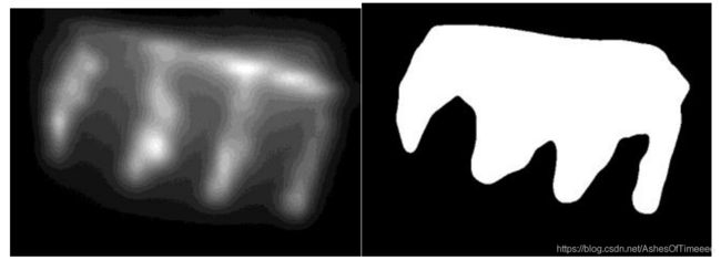
图左示出了初始重建结果的显著性映射inits，图右显示了二进制显著映射Winit。

2.3将Xinit分为n个块。基于Winit，如果至少图像块的五分之一的是白色的，则将此图像块视为显著性块；否则，将此图像块视为不显著的。
2.3.1图像分块
原理：图像分块的方法有很多，因为会遇到图片的长宽不能整除问题，这里用的是图像缩放法，如果用四舍五入法会导致判断显著性块的时候不准确。
图片缩放法：图像缩放一下，让其满足整除关系即可。

def display_blocks(divide_image):#  显示分块图片  
    m,n=divide_image.shape[0],divide_image.shape[1]
    for i in range(m):
        for j in range(n):
            plt.subplot(m,n,i*n+j+1)
            plt.imshow(divide_image[i,j,:])
            plt.show()
            plt.axis('off')
            plt.title('block:'+str(i*n+j+1))
def divide_method2(img,m,n):#分割成m行n列
    h, w = img.shape[0],img.shape[1]
    grid_h=int(h*1.0/(m-1)+0.5)#每个网格的高
    grid_w=int(w*1.0/(n-1)+0.5)#每个网格的宽
    
    #满足整除关系时的高、宽
    h=grid_h*(m-1)
    w=grid_w*(n-1)
    
    #图像缩放
    img_re=cv2.resize(img,(w,h),cv2.INTER_LINEAR)# 也可以用img_re=skimage.transform.resize(img, (h,w)).astype(np.uint8)
    #plt.imshow(img_re)
    gx, gy = np.meshgrid(np.linspace(0, w, n),np.linspace(0, h, m))
    gx=gx.astype(np.int)
    gy=gy.astype(np.int)

    divide_image = np.zeros([m-1, n-1, grid_h, grid_w,3], np.uint8)#这是一个五维的张量，前面两维表示分块后图像的位置（第m行，第n列），后面三维表示每个分块后的图像信息
    
    for i in range(m-1):
        for j in range(n-1):      
            divide_image[i,j,...]=img_re[
            gy[i][j]:gy[i+1][j+1], gx[i][j]:gx[i+1][j+1],:]
    return divide_image

将Xinit和Winit分别进行分块，分块后的图片命名为Xn和Wn并保存下来。
下面是X1------ X12



下面是W1----W12



2.3.1判断Wn白色区域是否大于1/5，如果大于等于1/5，则相应的Xn判定为显著图块。

def ostu(img):    #判断白色区域的占比
    a=len(img.astype(np.int8)[img==0])  #白色
    b=len(img.astype(np.int8)[img==1])  #黑色
    print(a*1.0/(a+b))

如果ostu（Wn）>=0.2,则对应的Xn为显著图块，保存下来，对这些图块进行下一步运算。

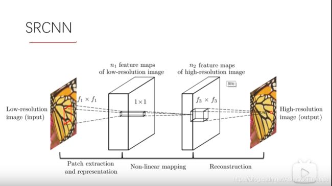
step3：基于SRCNN的超分辨率重建

srcnn是第一个使用深度学习，也是第一个使用卷积神经网络来解决超分辨率重建问题的。他的思路其实非常的简单：

step1：
首先将一张低分辨率图像进行一个插值的放大（双三次），放大成一个更大的低分辨率图像。
utils.py(主要进行预处理，前面已经做过，这里略)
step2：将低分辨率图像输入三层卷积神经网络：
2.1
图像块的提取和特征表示，利用卷积网络的性质提取图像块的特征:
经过99的一个卷积层，卷积核数目64 (n1),再经过relu层的激活，来提取特征。
F1(Y) = max(0,W1 ∗Y + B1) W1是滤波器；B1是偏差。
2.2
线性映射。将第一步的n1维特征映射到n2维
提取特征完了之后再经过这个11的卷积层和一个激活函数来进行映射。
F2(Y) = max(0,W2 ∗F1(Y) + B2)
2.3
重构。再做一次卷积进行重构，类似于传统方法的平均处理
最后我们再输入到这个5*5的卷积层里面，还有relu层，就重建出了一张SR图片。
F(Y) = W3 ∗F2(Y) + B3 B3是一个c维向量

pytorch版本的SRCNN代码一共分为3个.py文件，结构如下：
· models.py
· main.py
· utils.py

文件1: utils.py
简介：主要是用来进行预处理操作的。
方法总结：
def read_data(path): 读取h5格式数据文件，将其转换成np.array格式。
def preprocess(path, scale=3): 预处理单个图像文件（三插值）。
def prepare_data(sess, dataset): 得到当前文件路径。
def make_data(sess, data, label): 制作h5文件。
def imread(path, is_grayscale=True): 以YCbCr格式读取图像。
def modcrop(image, scale=3): 将图片规整到可以被scale整除的宽高。
def input_setup(sess, config): 就是把输入和输出图片，切成一小块存起来。
def imsave(image, path): 保存图片。
def merge(images, size): 将一个batch内的图片拼接在一起。

import os
import glob
import h5py
import random
import matplotlib.pyplot as plt

from PIL import Image  # for loading images as YCbCr format
import scipy.misc
import scipy.ndimage
import numpy as np

import tensorflow as tf

try:
  xrange #处理异常中断
except:
  xrange = range
  
FLAGS = tf.app.flags.FLAGS#命令行参数传递

def read_data(path):
  """
  Read h5 format data file
  读取h5文件中的data和label数据，需要将其转换成np.array格式
  Args:
    path: file path of desired file
    data: '.h5' file format that contains train data values
    label: '.h5' file format that contains train label values
  """
   #读取h5格式数据文件(用于训练或测试)
  with h5py.File(path, 'r') as hf:
    data = np.array(hf.get('data'))
    label = np.array(hf.get('label'))
    return data, label

def preprocess(path, scale=3):
  """
处理图片，input_,label_分别是输入和输出的图片，对应低分辨率和高分辨率
   预处理单个图像文件
     （1）以YCbCr格式读取原始图像（默认为灰度）
     （2）归一化  (将0-255的uint8型数据转换到0-1之间)
     （3）应用三次插值的图像文件

  Args:
    path: file path of desired file
    input_: image applied bicubic interpolation (low-resolution)
    label_: image with original resolution (high-resolution)
  """
  image = imread(path, is_grayscale=True)#以YCbCr格式读取图像。
  label_ = modcrop(image, scale) #将图片规整到可以被scale整除的宽和高

  # Must be normalized
  image = image / 255.
  label_ = label_ / 255.

'''
scipy.ndimage.interpolation.zoom(
      input,  #输入数组
      zoom,   #沿轴的缩放系数。
      output=None,  #放置输出的数组，或返回数组的dtype
      order=3,      #样条插值的顺序(0～5)，=3:三次插值，=0:最近插值，=1:双线性插值.
      mode='constant', #根据给定的模式（'常数'，'最近'，'反映'或'换行'）填充输入边界之外的点
      cval=0.0,        #如果mode ='constant'，则用于输入边界之外的点的值。
      prefilter=True)  #是否在插值之前使用spline_filter进行预过滤，如果为False，则假定输入已被过滤。
'''
#两次插值,先缩小再扩大。
#使用三次插值缩小scale倍
  input_ = scipy.ndimage.interpolation.zoom(label_, (1./scale), prefilter=False)
#使用三次插值扩大scale倍
  input_ = scipy.ndimage.interpolation.zoom(input_, (scale/1.), prefilter=False)

  return input_, label_  #低分辨率，高分辨率(195,174,1)

def prepare_data(sess, dataset):
  """
得到图片路径list
  Args:
    dataset: choose train dataset or test dataset
    
    For train dataset, output data would be ['.../t1.bmp', '.../t2.bmp', ..., '.../t99.bmp']
  """
  if FLAGS.is_train:
    filenames = os.listdir(dataset)  #os.getcwd():得到当前文件路径
    data_dir = os.path.join(os.getcwd(), dataset)
    data = glob.glob(os.path.join(data_dir, "*.bmp"))
  else:
    data_dir = os.path.join(os.sep, (os.path.join(os.getcwd(), dataset)), "Set5")
    data = glob.glob(os.path.join(data_dir, "*.bmp"))

  return data

def make_data(sess, data, label):
  """
  制作h5文件，将data（checkpoint下的train.h5 或test.h5）利用h5的create_dataset 写入
  Make input data as h5 file format
  Depending on 'is_train' (flag value), savepath would be changed.
  将输入数据设置为h5文件格式
  根据“ is_train”（标志值），保存路径将被更改。
  """
  if FLAGS.is_train:
    savepath = os.path.join(os.getcwd(), 'checkpoint/train.h5')#定义h5文件保存地址
  else:
    savepath = os.path.join(os.getcwd(), 'checkpoint/test.h5')

  with h5py.File(savepath, 'w') as hf:
    hf.create_dataset('data', data=data)#建立一个名叫"data"的HDF5数据集
    hf.create_dataset('label', data=label)#建立一个名叫"label"的HDF5数据集
#以YCbCr格式读取图像
def imread(path, is_grayscale=True):
  """
  Read image using its path.
  Default value is gray-scale, and image is read by YCbCr format as the paper said.
  """
  if is_grayscale:
    return scipy.misc.imread(path, flatten=True, mode='YCbCr').astype(np.float)
  else:
    return scipy.misc.imread(path, mode='YCbCr').astype(np.float)

def modcrop(image, scale=3):
  """
将图片规整到可以被scale整除的宽高。
  To scale down and up the original image, first thing to do is to have no remainder while scaling operation.
  
  We need to find modulo of height (and width) and scale factor.
  Then, subtract the modulo from height (and width) of original image size.
  There would be no remainder even after scaling operation.
  要按比例放大和缩小原始图像，首先要做的是在缩放操作时没有余数。 
   我们需要找到高度（和宽度）和比例因子的模。
   然后，从原始图像尺寸的高度（和宽度）中减去模。
   即使在缩放操作之后也将没有剩余。
  """
  if len(image.shape) == 3: 
    h, w, _ = image.shape  #eg: image.shape=(197, 176, 3), scale=3
    h = h - np.mod(h, scale)#h=195
    w = w - np.mod(w, scale)#w=174
    image = image[0:h, 0:w, :]
  else:
    h, w = image.shape
    h = h - np.mod(h, scale)
    w = w - np.mod(w, scale)
    image = image[0:h, 0:w]
  return image
#测试时返回每行每列能裁剪出的子图个数
def input_setup(sess, config):
  """
  就是把输入和输出图片，切成一小块存起来
  Read image files and make their sub-images and saved them as a h5 file format.
  读取图像文件并制作其子图像，并将其保存为h5文件格式。
  """
  # Load data path
  if config.is_train:
    data = prepare_data(sess, dataset="Train")#图的位置列表
  else:
    data = prepare_data(sess, dataset="Test")

  sub_input_sequence = []
  sub_label_sequence = []
  padding = abs(config.image_size - config.label_size) / 2 # (33-21)/2=6

  if config.is_train: #对于每张图
    for i in xrange(len(data)):
      input_, label_ = preprocess(data[i], config.scale) #预处理 低分辨率，高分辨率

      if len(input_.shape) == 3:
        h, w, _ = input_.shape  #195,174,1
      else:
        h, w = input_.shape

      for x in range(0, h-config.image_size+1, config.stride): #(0~163)
        for y in range(0, w-config.image_size+1, config.stride): #(0~142)
           # (x ~ x+33, y ~ y+33),裁剪成[33*33]的小图
          sub_input = input_[x:x+config.image_size, y:y+config.image_size]
           # (x+6 ~ x+6+21，y+6 ~ y+6+21),裁剪成[21*21]的小图，舍弃边缘部分
          sub_label = label_[x+int(padding):x+int(padding)+config.label_size, y+int(padding):y+int(padding)+config.label_size] # [21 x 21]

          # 重定义图片块大小
          sub_input = sub_input.reshape([config.image_size, config.image_size, 1])#image_size：33，即33*33*1
          sub_label = sub_label.reshape([config.label_size, config.label_size, 1]) #label_size：21，即21*21*1

          sub_input_sequence.append(sub_input)#将小图添加到输入列表
          sub_label_sequence.append(sub_label)#将小图添加到标签列表

  else:#test只对其中的一张图片做处理。
    input_, label_ = preprocess(data[2], config.scale)

    if len(input_.shape) == 3:
      h, w, _ = input_.shape
    else:
      h, w = input_.shape

    # Numbers of sub-images in height and width of image are needed to compute merge operation.
    # 计算合并操作需要图像高度和宽度中的子图像数量。
    nx = ny = 0 
    for x in range(0, h-config.image_size+1, config.stride):
      nx += 1; ny = 0
      for y in range(0, w-config.image_size+1, config.stride):
        ny += 1
        sub_input = input_[x:x+config.image_size, y:y+config.image_size] # [33 x 33]
        sub_label = label_[x+int(padding):x+int(padding)+config.label_size, y+int(padding):y+int(padding)+config.label_size] # [21 x 21]
        
        sub_input = sub_input.reshape([config.image_size, config.image_size, 1])  
        sub_label = sub_label.reshape([config.label_size, config.label_size, 1])

        sub_input_sequence.append(sub_input)
        sub_label_sequence.append(sub_label)

  """
  len(sub_input_sequence) : the number of sub_input (33 x 33 x ch) in one image
  (sub_input_sequence[0]).shape : (33, 33, 1)
  """
  # Make list to numpy array. With this transform
  #需要将数据转成numpy类型，被存为h5格式
  arrdata = np.asarray(sub_input_sequence) # [?, 33, 33, 1]
  arrlabel = np.asarray(sub_label_sequence) # [?, 21, 21, 1]

  make_data(sess, arrdata, arrlabel)

  if not config.is_train:
    return nx, ny

#保存图片   
def imsave(image, path):
  return scipy.misc.imsave(path, image)
"""
  将一个batch内的图片拼接在一起
  images：一个batch图片，
  size：第一个参数是高度上有几张图片，第二个宽度上有几张图片
  %：求模运算，取余。
  //：取整，返回不大于结果的一个最大的整数
  /：浮点数除法
  """
def merge(images, size):
  h, w = images.shape[1], images.shape[2]
  img = np.zeros((h*size[0], w*size[1], 1))
  for idx, image in enumerate(images):
    i = idx % size[1]
    j = idx // size[1]
    img[j*h:j*h+h, i*w:i*w+w, :] = image

  return img

文件2：models,py
简介：主要用来制作网络的。
方法总结：
class SRCNN(object): 初始化SRCNN类。
def build_model(self): 创建网络。
def train(self, config): 训练或测试网络。
def model(self): 网络结构。
*def save(self, checkpoint_dir, step):*存储sess。
def load(self, checkpoint_dir): 加载sess，成功加载返回True，否则返回False。

from utils import (
  read_data, 
  input_setup, 
  imsave,
  merge
)

import time
import os
import matplotlib.pyplot as plt

import numpy as np
import tensorflow as tf

try:
  xrange
except:
  xrange = range

class SRCNN(object):  #SRCNN对象初始化设置

  def __init__(self, 
               sess, 
               image_size=33,
               label_size=21, 
               batch_size=128,
               c_dim=1, 
               checkpoint_dir=None, 
               sample_dir=None):

    self.sess = sess
    self.is_grayscale = (c_dim == 1)
    self.image_size = image_size
    self.label_size = label_size
    self.batch_size = batch_size

    self.c_dim = c_dim

    self.checkpoint_dir = checkpoint_dir
    self.sample_dir = sample_dir
    self.build_model()

'''
三次卷积，卷积核大小分别是9，1，5。输出通道分别是64，32，1。
    #第一层CNN：对输入图片的特征提取。（9 x 9 x 64卷积核）
    #第二层CNN：对第一层提取的特征的非线性映射（1 x 1 x 32卷积核）
    #第三层CNN：对映射后的特征进行重建，生成高分辨率图像（5 x 5 x 1卷积核）
'''
#创建网络
  def build_model(self):
# 插入一个将始终供给张量的占位符（张量的元素类型, shape=要输入的张量的形状（可选）, name=操作的名称（可选））
    self.images = tf.placeholder(tf.float32, [None, self.image_size, self.image_size, self.c_dim], name='images')
    self.labels = tf.placeholder(tf.float32, [None, self.label_size, self.label_size, self.c_dim], name='labels')
    
    self.weights = {
      'w1': tf.Variable(tf.random_normal([9, 9, 1, 64], stddev=1e-3), name='w1'),
      'w2': tf.Variable(tf.random_normal([1, 1, 64, 32], stddev=1e-3), name='w2'),
      'w3': tf.Variable(tf.random_normal([5, 5, 32, 1], stddev=1e-3), name='w3')
    }
#偏置
    self.biases = {
      'b1': tf.Variable(tf.zeros([64]), name='b1'),
      'b2': tf.Variable(tf.zeros([32]), name='b2'),
      'b3': tf.Variable(tf.zeros([1]), name='b3')
    }

    self.pred = self.model()#只要调用了model函数就会有输出，返回三层卷积后的结果，预测值

    # Loss function (MSE)
    self.loss = tf.reduce_mean(tf.square(self.labels - self.pred))
# 主函数调用(训练或测试)，创建一个Saver变量
    self.saver = tf.train.Saver()

  def train(self, config):
#读取图像文件并制作其子图像，并将其保存为h5文件格式。
    if config.is_train:
      input_setup(self.sess, config)
    else:
      nx, ny = input_setup(self.sess, config)
# 训练为checkpoint下train.h5；测试为checkpoint下test.h5
    if config.is_train:     
      data_dir = os.path.join('./{}'.format(config.checkpoint_dir), "train.h5")
    else:
      data_dir = os.path.join('./{}'.format(config.checkpoint_dir), "test.h5")

    train_data, train_label = read_data(data_dir)

#建立优化器，初始化所有参数，计数器，计时器
#这里采用SGD（具有标准反向传播的随机梯度下降）优化器。还有Adam优化器，据说SGD的效果更好（待验证）
    self.train_op = tf.train.GradientDescentOptimizer(config.learning_rate).minimize(self.loss)

    tf.initialize_all_variables().run()
    
    counter = 0#计数器
    start_time = time.time()#计时器
 #加载训练过的参数
    if self.load(self.checkpoint_dir):
      print(" [*] Load SUCCESS")
    else:
      print(" [!] Load failed...")
 #训练模型，每隔500次保存一次模型
    if config.is_train:
      print("Training...")

      for ep in xrange(config.epoch):
        # Run by batch images
        batch_idxs = len(train_data) // config.batch_size#计算一个epoch有多少batch
        for idx in xrange(0, batch_idxs): #以batch为单元更新
          batch_images = train_data[idx*config.batch_size : (idx+1)*config.batch_size]
          batch_labels = train_label[idx*config.batch_size : (idx+1)*config.batch_size]

          counter += 1
          _, err = self.sess.run([self.train_op, self.loss], feed_dict={self.images: batch_images, self.labels: batch_labels})

          if counter % 10 == 0:#每更新10次输出一次数据
            print("Epoch: [%2d], step: [%2d], time: [%4.4f], loss: [%.8f]" \
              % ((ep+1), counter, time.time()-start_time, err))

          if counter % 500 == 0:#每更新500次保存一次数据
            self.save(config.checkpoint_dir, counter)

    else:
      print("Testing...")
      #执行前面所有的操作
      rersult = self.pred.eval({self.images: train_data, self.labels: train_label})
      result = merge(result, [nx, ny])#将一个batch内的图片拼接在一起，测试时只切一张图所以一个batch就是全部输入
      result = result.squeeze()#squeeze去除维度为1的地方
      #保存图片
      image_path = os.path.join(os.getcwd(), config.sample_dir)#生成保存地址
      image_path = os.path.join(image_path, "test_image.png")#保存地址/图片名
      imsave(result, image_path)#保存图片

  def model(self):
     '''
    将图片经过3次卷积，步长都是1。
    卷积加偏置，前两层有relu激活函数，最后一层无激活函数。
    :return: 最后的一次的卷积结果

    strides在官方定义中是一个一维具有四个元素的张量，
    其规定前后必须为1，所以我们可以改的是中间两个数，
    中间两个数分别代表了水平滑动和垂直滑动步长值。
    '''
    conv1 = tf.nn.relu(tf.nn.conv2d(self.images, self.weights['w1'], strides=[1,1,1,1], padding='VALID') + self.biases['b1'])
    conv2 = tf.nn.relu(tf.nn.conv2d(conv1, self.weights['w2'], strides=[1,1,1,1], padding='VALID') + self.biases['b2'])
    conv3 = tf.nn.conv2d(conv2, self.weights['w3'], strides=[1,1,1,1], padding='VALID') + self.biases['b3']
    return conv3

#确认路径，存储sess
  def save(self, checkpoint_dir, step):
    model_name = "SRCNN.model"
    model_dir = "%s_%s" % ("srcnn", self.label_size)
    checkpoint_dir = os.path.join(checkpoint_dir, model_dir)

    if not os.path.exists(checkpoint_dir):
        os.makedirs(checkpoint_dir)
'''
    向文件夹中写入包含当前模型中所有可训练变量的checkpoint文件，
    之后可以使用saver.restore()方法，重载模型的参数，继续训练或者用于测试数据
'''
    self.saver.save(self.sess,
                    os.path.join(checkpoint_dir, model_name),
                    global_step=step)
#加载sess，成功加载返回True，否则返回False。
  def load(self, checkpoint_dir):
    print(" [*] Reading checkpoints...")
    model_dir = "%s_%s" % ("srcnn", self.label_size)
    checkpoint_dir = os.path.join(checkpoint_dir, model_dir)

    ckpt = tf.train.get_checkpoint_state(checkpoint_dir) #从文件夹中获取checkpoint文件
    if ckpt and ckpt.model_checkpoint_path:
        ckpt_name = os.path.basename(ckpt.model_checkpoint_path)#获取checkpoint文件的文件名
        self.saver.restore(self.sess, os.path.join(checkpoint_dir, ckpt_name))#重载模型的参数，继续训练或者用于测试数据
        return True
    else:
        return False

文件3：main.py
简介：主函数
方法总结：

from model import SRCNN
from utils import input_setup
import numpy as np
import tensorflow as tf
import h5py
import pprint
import os
'''
定义训练和测试参数
（如果采用SGD优化器时的bschsize，学习率，步长stride，训练或测试模式）
此后由设定的参数进行训练或者测试。
'''
flags = tf.app.flags
#命令行执行时传参数，使用命令行运行的时候可以定义参数
#参数名称/默认值/参数描述
flags.DEFINE_integer("epoch", 15000, "Number of epoch [15000]")
flags.DEFINE_integer("batch_size", 128, "The size of batch images [128]")
flags.DEFINE_integer("image_size", 33, "The size of image to use [33]")
#因为卷积时不进行padding，3层卷积后特征尺寸变为21，为此将图像中心的21*21的小图像作为标签
flags.DEFINE_integer("label_size", 21, "The size of label to produce [21]")
flags.DEFINE_float("learning_rate", 1e-4, "The learning rate of gradient descent algorithm [1e-4]")
#图像颜色维度
flags.DEFINE_integer("c_dim", 1, "Dimension of image color. [1]")
#3次插值时的尺度
flags.DEFINE_integer("scale", 3, "The size of scale factor for preprocessing input image [3]")
#卷积的步长
flags.DEFINE_integer("stride", 14, "The size of stride to apply input image [14]")
flags.DEFINE_string("checkpoint_dir", "checkpoint", "Name of checkpoint directory [checkpoint]")
flags.DEFINE_string("sample_dir", "sample", "Name of sample directory [sample]")
flags.DEFINE_boolean("is_train", True, "True for training, False for testing [True]")
FLAGS = flags.FLAGS

pp = pprint.PrettyPrinter()

def main(_):
  pp.pprint(flags.FLAGS.__flags)

  if not os.path.exists(FLAGS.checkpoint_dir):
    os.makedirs(FLAGS.checkpoint_dir) #在当前地址创建“checkpoint”文件夹
  if not os.path.exists(FLAGS.sample_dir):
    os.makedirs(FLAGS.sample_dir) #在当前地址创建“sample”文件夹

  with tf.Session() as sess:
    srcnn = SRCNN(sess, 
                  image_size=FLAGS.image_size, 
                  label_size=FLAGS.label_size, 
                  batch_size=FLAGS.batch_size,
                  c_dim=FLAGS.c_dim, 
                  checkpoint_dir=FLAGS.checkpoint_dir,
                  sample_dir=FLAGS.sample_dir) #创建一个SRCNN对象，自动调用初始化函数

    srcnn.train(FLAGS)
    
if __name__ == '__main__':   #import到其他脚本中不会被执行

	CNN网络没有包含池化层和全连接层
	损失函数：均方误差（Mean Squared Error，MSE)

将SRCNN分别应用于每个显著图像块
综上，显著图块为：
X1—X8 和X12

效果

结果图片

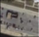
对比
原始图像：

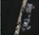
result of ours:

可以看出效果还是比较明显的。

PS:
其实上文中有些图片是直接引用的论文中的图片。还有srcnn的代码我的电脑python版本不对应，所以srcnn的代码我是用原版matlab代码，让LH同学帮忙生成了一个灰度图片：

其实SRCNN的效果并不是十分明显的，现在有很多更好的网络比如GAN网络等可以实现更好的超分辨率效果，这篇论文本质上是提出了一种方法：在图片分辨率要求不是过高的情况下，采用提取显著块的方法可以更快，提高效率。
下面是文章中提到的运行时间对比：

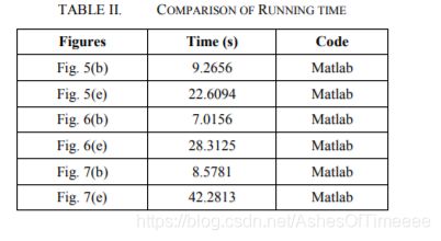
所以如果你想提高效率，可以考虑引入本文中“斑块“的概念。

PSS:
另外，我发现SRCNN和预处理的代码对图片尺寸要求比较严格，已经通道数也要注意，不然会报错。