【论文阅读】SML：标准最大logits

Standardized Max Logits: A Simple yet Effective Approach for Identifying Unexpected Road Obstacles in Urban-Scene Segmentation
标准max logit：在城市场景分割中识别意外道路障碍的一种简单但有效的方法

论文翻译

Abstract

Identifying unexpected objects on roads in semantic seg- mentation (e.g., identifying dogs on roads) is crucial in safety-critical applications. Existing approaches use images of unexpected objects from external datasets or re- quire additional training (e.g., retraining segmentation networks or training an extra network), which necessitate a non-trivial amount of labor intensity or lengthy inference time. One possible alternative is to use prediction scores of a pre-trained network such as the max logits (i.e., maximum values among classes before the final softmax layer) for detecting such objects. However, the distribution of max logits of each predicted class is significantly different from each other, which degrades the performance of identifying un- expected objects in urban-scene segmentation. To address this issue, we propose a simple yet effective approach that* standardizes the max logits in order to align the different distributions and reflect the relative meanings of max log- its within each predicted class. Moreover, we consider the local regions from two different perspectives based on the intuition that neighboring pixels share similar semantic in- formation. In contrast to previous approaches, our method does not utilize any external datasets or require additional training, which makes our method widely applicable to ex-isting pre-trained segmentation models. Such a straightfor- ward approach achieves a new state-of-the-art performance on the publicly available Fishyscapes Lost & Found leader- board with a large margin. Our code is publicly available at this link 1.

在语义分割中识别道路上的意外物体（例如，识别道路上的狗）在安全关键型应用中至关重要。

现有方法：

• 使用来自外部数据集的意外对象的图像或需要额外的训练（重新训练分割网络或训练额外的网络）

  缺点：需要大量的劳动强度或冗长的推理时间

• 预训练网络的预测分数（例如maxlogit，最终 softmax 层之前的类之间的最大值）

  缺点：每个预测类别的最大 logits 分布彼此之间存在显着差异，这降低了在城市场景分割中识别非预期对象的性能

改进：

1. 标准化 max logits：对齐不同的分布并反映每个预测类别中 max logits 的相对含义。
2. 基于相邻像素共享相似语义信息的直觉，从两个不同的角度考虑局部区域。

标准maxlogit优势：不使用任何外部数据集或需要额外的训练，广泛适用于现有的预训练分割模型。

结果：在公开可用的 Fishyscapes Lost & Found 排行榜上实现了新的最先进的性能，并有很大的优势。

1. Introduction

Recent studies [8, 9, 22, 40, 43, 44, 12] in semantic segmentation focus on improving the segmentation per- formance on urban-scene images. Despite such recent ad- vances, these approaches cannot identify unexpected ob- jects (i.e., objects not included in the pre-defined classes during training), mainly because they predict all the pixels as one of the pre-defined classes. Addressing such an is- sue is critical especially for safety-critical applications such as autonomous driving. As shown in Fig. 1, wrongly pre- dicting a dog (i.e., an unexpected object) on the road as the road does not stop the autonomous vehicle, which may lead to roadkill. In this safety-critical point of view, the dog should be detected as an unexpected object which works as the starting point of the autonomous vehicle to handle these objects differently (e.g., whether to stop the car or circumvent the dog).

近期提升城市场景图像语义分割性能的研究：¹, ²,³, ⁴, ⁵, ⁶, ⁷

这些方法不足之处：无法识别意外对象（即训练期间未包含在预定义类中的对象）

原因：将所有像素预测为预定义类之一

解决此类问题至关重要，尤其是对于自动驾驶等安全关键型应用。 如图 1 所示，错误地将道路上的狗（即意外物体）预测为道路不会停止自动驾驶汽车，这可能会导致道路死亡。 从这个安全关键的角度来看，狗应该被检测为一个意外的物体，它作为自动驾驶汽车的起点，以不同的方式处理这些物体（例如，是停下汽车还是绕过狗）。

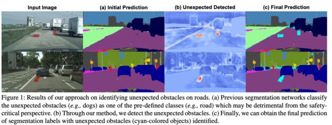
图1：我们识别道路上意外障碍物的方法的结果。
(a) 先前的分割网络将意外的障碍物（例如狗）分类为预定义的类别（例如道路）之一，这从安全关键的角度来看可能是有害的。
(b) 通过我们的方法，我们检测到了意外的障碍。
© 最后，我们可以获得识别出意外障碍物（青色物体）的分割标签的最终预测。

Several studies [3, 26, 25, 5, 35, 2, 14] tackle the problem of detecting such unexpected objects on roads. Some approaches [2, 5] utilize external datasets [36, 24] as samples of unexpected objects while others [26, 39, 25, 33] leverage image resynthesis models for erasing the regions of such objects. However, such approaches require a considerable amount of labor intensity or necessitate a lengthy inference time. On the other hand, simple approaches which leverage only a pre-trained model [18, 23, 20] are proposed for out-of-distribution (OoD) detection in image classification, the task of detecting images from a different distribution compared to that of the train set. Based on the intuition that a correctly classified image generally has a higher maximum softmax probability (MSP) than an OoD image [18], MSP is used as the anomaly score (i.e., the value used for detecting OoD samples). Alternatively, utilizing the max logit [16] (i.e., maximum values among classes before the final soft- max layer) as the anomaly score is proposed, which out- performs using MSP for detecting anomalous objects in se- mantic segmentation. Note that high prediction scores (e.g., MSP and max logit) indicate low anomaly scores and vice versa.

在道路上检测此类意外物体的问题的几项研究 [3, 26, 25, 5, 35, 2, 14] 。

• [2, 5] 利用外部数据集 [36, 24] 作为意外对象的样本，

• [26, 39, 25, 33] 利用图像再合成模型来擦除这些对象的区域。 然而，这种方法需要大量的劳动强度或需要很长的推理时间。

• 仅利用预训练模型 [18,23,20] 的简单方法用于图像分类中的分布外 (OoD) 检测，检测与训练集相比不同分布的图像。

• 基于正确分类的图像通常具有比 OoD 图像 [18] 更高的最大 softmax 概率 (MSP) 的直觉，MSP 被用作异常分数（用于检测 OoD 样本的值)

• 提出了利用最大 logit [16]（最终 softmax 层之前的类之间的最大值）作为异常分数，其在语义分割中使用 MSP 检测异常对象的性能优于使用 MSP 检测异常对象。

请注意，高预测分数（例如， MSP 和最大 logit）表示低异常分数，反之亦然。

However, directly using the MSP [18] or the max logit [16] as the anomaly score has the following limita- tions. Regarding the MSP [18], the softmax function has the fast-growing exponential property which produces highly confident predictions. Pre-trained networks may be highly confident with OoD samples which limits the performance of using MSPs for detecting the anomalous samples [23]. In the case of the max logit [16], as shown in Fig. 2, the val- ues of the max logit have their own ranges in each predicted class. Due to this fact, the max logits of the unexpected ob- jects predicted as particular classes (e.g., road) exceed those of other classes (e.g., train) in the in-distribution objects. This can degrade the performance of detecting unexpected objects on evaluation metrics (e.g., AUROC and AUPRC) that use the same threshold for all classes.

直接使用 MSP [18] 或最大 logit [16] 作为异常分数的限制：

• MSP [18]：softmax 函数具有快速增长的指数特性，可以产生高度可信的预测。 预训练的网络可能对 OoD 样本高度自信，这限制了使用 MSP 检测异常样本的性能 [23]。

• 最大 logit [16] ：如图 2 所示，最大 logit 的值在每个预测类别中都有自己的范围。 由于这个事实，预测为特定类（例如，道路）的意外对象的最大 logits 超过了分布对象中其他类（例如，火车）的最大 logits。 这会降低在对所有类使用相同阈值的评估指标（例如 AUROC 和 AUPRC）上检测意外对象的性能。

图 2：Fishyscapes Static 中的 MSP、最大 logit 和标准化最大 logit 的箱线图。 X 轴表示在训练阶段按像素出现次数排序的类。 Y 轴表示每种方法的值。 红色和蓝色分别代表分布内像素和意外像素中的值分布。 每个条的下限和上限表示 Q1 和 Q3，而点表示其预测类别的平均值。 灰色表示两组的重叠区域。 灰色区域的不透明度与 TPR 95% 时的 FPR 成正比。 以分类方式标准化最大 logits 明显降低了 FPR。

In this work, inspired by this finding, we propose standardizing the max logits in a class-wise manner, termed standardized max logits (SML). Standardizing the max log- its aligns the distributions of max logits in each predicted class, so it enables to reflect the relative meanings of val- ues within a class. This reduces the false positives (i.e., in-distribution objects detected as the unexpected objects, highlighted as gray regions in Fig. 2) when using a single threshold.

在这项工作中，受这一发现的启发，我们建议以分类方式对最大 logits 进行标准化，称为 standardized max logits (SML)。 标准化最大对数会对齐每个预测类中最大对数的分布，因此它能够反映类内值的相对含义。 当使用单个阈值时，这减少了误报（被检测为意外对象的分布中对象，在图 2 中突出显示为灰色区域）。

Moreover, we further improve the performance of identifying unexpected obstacles using the local semantics from two different perspectives. First, we remove the false positives in boundary regions where predicted class changes from one to another. Due to the class changes, the boundary pixels tend to have low prediction scores (i.e., high anomaly scores) compared to the non-boundary pixels [38, 1]. In this regard, we propose a novel iterative boundary sup- pression to remove such false positives by replacing the high anomaly scores of boundary regions with low anomaly scores of neighboring non-boundary pixels. Second, in order to remove the remaining false positives in both bound- ary and non-boundary regions, we smooth them using the neighboring pixels based on the intuition that local consistency exists among the pixels in a local region. We term this process as dilated smoothing.

此外，我们从两个不同的角度进一步提高了使用局部语义识别意外障碍物的性能。

1. 在预测的类从一个到另一个变化的边界区域中删除了误报。 由于类别变化，与非边界像素相比，边界像素往往具有较低的预测分数（即高异常分数）[38, 1]。 在这方面，我们提出了一种新的迭代边界抑制，通过用相邻非边界像素的低异常分数替换边界区域的高异常分数来消除这种误报。

   怎么确定边界的？

2. 为了消除边界和非边界区域中剩余的误报，根据局部区域中像素之间存在局部一致性的直觉，使用相邻像素对它们进行平滑处理。 将此过程称为扩张平滑。

相邻像素，好像非极大抑制啊

The main contributions of our work are as follows:

• We propose a simple yet effective approach for identi- fying unexpected objects on roads in urban-scene se- mantic segmentation.
• Our proposed approach can easily be applied to vari- ous existing models since our method does not require additional training or external datasets.
• We achieve a new state-of-the-art performance on the publicly available Fishyscapes Lost & Found Leader- board2 among the previous approaches with a large margin and negligible computation overhead while not requiring additional training and OoD data.

主要贡献：

• 提出了一种简单而有效的方法，用于在城市场景语义分割中识别道路上的意外物体。
• 本方法可以很容易地应用于各种现有模型，因为不需要额外的训练或外部数据集。
• 在公开可用的 Fishyscapes Lost & Found Leaderboard2 上实现了新的最先进的性能（以前的方法中具有很大的余量和可忽略的计算开销）同时不需要额外的训练和 OoD 数据。

2. Related Work

2.1. Semantic segmentation on urban driving scenes

Recent studies [8, 9, 22, 40, 43, 44, 12, 6, 34, 32] have strived to enhance the semantic segmentation performance on urban scenes. The studies [22, 40] consider diverse scale changes in urban scenes or leverage the innate geometry and positional patterns found in urban-scene images [9]. Moreover, several studies [6, 34, 32] have proposed more efficient architectures to improve the inference time, which is critical for autonomous driving. Despite the advances, unex- pected objects cannot be identified by these models, which is another important task for safetycritical applications. Regarding the importance of such a task from the safetycritical perspective, we focus on detecting unexpected ob- stacles in urban-scene segmentation.

最近的研究 [8, 9, 22, 40, 43, 44, 12, 6, 34, 32] 致力于提高城市场景的语义分割性能。 研究 [22, 40] 考虑了城市场景中的不同尺度变化或利用城市场景图像中发现的先天几何和位置模式 [9]。 此外，一些研究 [6, 34, 32] 提出了更有效的架构来改善推理时间，这对于自动驾驶至关重要。 尽管取得了进步，但这些模型无法识别意外对象，这是安全关键应用程序的另一项重要任务。 从安全关键的角度来看，这项任务的重要性，我们专注于检测城市场景分割中的意外障碍。

2.2. Detecting unexpected objects in semantic segmentation 在语义分割中检测意外对象

Several studies [2, 5, 3] utilize samples of unexpected objects from external datasets during the training phase. For example, by assuming that the objects cropped from the Im- ageNet dataset [36] are anomalous objects, they are overlaid on original training images [2] (e.g., Cityscapes) to provide samples of unexpected objects. Similarly, another previous work [5] utilizes the objects from the COCO dataset [24] as samples of unexpected objects. However, such meth- ods require retraining the network by using the additional datasets, which hampers to utilize a given pre-trained seg- mentation network directly.

Other work [26, 39, 25, 33] exploits the image resynthesis (i.e., reconstructing images from segmentation predic- tions) for detecting unexpected objects. Based on the intu- ition that image resynthesis models fail to reconstruct the regions with unexpected objects, these studies use the dis- crepancy between an original image and the resynthesized image with such objects excluded. However, utilizing an ex- tra image resynthesis model to detect unexpected objects necessitates a lengthy inference time that is critical in semantic segmentation. In the real-world application of se- mantic segmentation (e.g., autonomous driving), detecting unexpected objects should be finalized in real-time. Consid- ering such issues, we propose a simple yet effective method that can be applied to a given segmentation model without requiring additional training or external datasets.

一些研究[2,5,3]在训练阶段利用来自外部数据集的意外对象样本。 例如，假设从 ImageNet 数据集 [36] 中裁剪的对象是异常对象，它们将覆盖在原始训练图像 [2]（例如 Cityscapes）上以提供意外对象的样本。 同样，之前的另一项工作 [5] 利用 COCO 数据集 [24] 中的对象作为意外对象的样本。 然而，这种方法需要通过使用额外的数据集来重新训练网络，这阻碍了直接利用给定的预训练分割网络。

其他工作 [26, 39, 25, 33] 利用图像重新合成（即从分割预测重建图像）来检测意外对象。 基于图像再合成模型无法重建具有意外物体的区域的直觉，这些研究使用了原始图像与排除这些物体的再合成图像之间的差异。 然而，利用额外的图像再合成模型来检测意外对象需要很长的推理时间，这在语义分割中至关重要。 在语义分割的实际应用中（例如，自动驾驶），应实时完成对意外对象的检测。 考虑到这些问题，我们提出了一种简单而有效的方法，可以应用于给定的分割模型，而不需要额外的训练或外部数据集。

3. Proposed Method

This section presents our approach for detecting unex- pected road obstacles. We first present how we standardize the max logits in Section 3.2 and explain how we consider the local semantics in Section 3.3.

本节介绍了我们检测意外道路障碍物的方法。 我们首先在 3.2 节介绍我们如何标准化最大 logits，并在 3.3 节解释我们如何考虑局部语义。

3.1. Method Overview

As our method overview is illustrated in Fig. 3, we first obtain the max logits and standardize them, based on the finding that the max logits have their own ranges according to the predicted classes. These different ranges cause unex- pected objects (pixels in blue boxes) predicted as a certain class to have higher max logit values (i.e., lower anomaly scores) than in-distribution pixels in other classes. This is- sue is addressed by standardizing the max logits in a class- wise manner since it enables to reflect the relative meanings within each predicted class.

由于我们的方法概述如图 3 所示，我们首先获得最大 logits 并标准化它们，基于最大 logits 根据预测类别有自己的范围的发现。 这些不同的范围导致预测为某个类别的意外对象（蓝色框中的像素）比其他类别中的分布内像素具有更高的最大 logit 值（较低的异常分数）。 这个问题是通过以类别方式标准化最大 logits 来解决的，因为它能够反映每个预测类别中的相对含义。

图 3：我们的方法概述。 我们从分割网络中获得最大 logits，并 (a) 使用从训练样本中获得的统计数据对其进行标准化。 (b) 然后，我们用周围的非边界像素迭代地替换边界区域的标准化最大 logits。 © 最后，我们应用扩张平滑来考虑广泛接受域中的局部语义。

Then, we remove the false positives (pixels in green boxes) in boundary regions. Generally, false positives in boundary pixels have lower prediction scores than neigh- boring in-distribution pixels. We reduce such false posi- tives by iteratively updating boundary pixels using anomaly scores of neighboring non-boundary pixels. Additionally, there exist a non-trivial number of pixels that have signif- icantly different anomaly scores compared to their neigh- boring pixels, which we term as irregulars (pixels in yellow boxes). Based on the intuition that local consistency (i.e., neighboring pixels sharing similar semantics) exists among pixels in a local region, we apply the smoothing filter with broad receptive fields. Note that we use the negative value of the final SML as the anomaly score.

然后，我们删除边界区域中的误报（绿色框中的像素） 通常，边界像素中的误报比相邻的分布内像素具有更低的预测分数。 我们通过使用相邻非边界像素的异常分数迭代更新边界像素来减少此类误报。 此外，存在大量像素与其相邻像素相比具有显着不同的异常分数，我们将其称为不规则像素（黄色框中的像素）。 基于局部一致性（相邻像素共享相似语义）存在于局部区域中的像素之间的直觉，我们应用具有广泛感受野的平滑滤波器。 请注意，我们使用最终 SML 的负值作为异常分数。

The following describes the process of how we obtain the max logit and the prediction at each pixel with a given image and the number of pre-defined classes. Let $X\in {\mathbb{R}}^{3\times H\times W}$ and $C$ denote the input image and the number of pre-defined classes, where H and W are the image height, and width, respectively. The logit output $F\in {\mathbb{R}}^{3\times H\times W}$ can be obtained from the segmentation network before the softmaxlayer.Then,themaxlogit $L\in {\mathbb{R}}^{H\times W}$ andprediction $\hat{Y}\in {\mathbb{R}}^{H\times W}$ at each location h, w are defined as

获得最大 logit 以及使用给定图像和预定义类的数量在每个像素处进行预测的过程:

$X\in {\mathbb{R}}^{3\times H\times W}$ 输入图像
$C$ 预定义类的数量
$H$ 和 $W$ 分别是图像的高度和宽度。

logit 输出 $F\in {\mathbb{R}}^{3\times H\times W}$ 可以在 softmax 层之前从分割网络中获得。

在每个位置 h，w 处的 maxlogit $L\in {\mathbb{R}}^{H\times W}$ 和预测 $\hat{Y}\in {\mathbb{R}}^{H\times W}$ 定义为
$$L_{h,w}=ma{x}_c{F}_{c,h,w}\text{\hspace{1em}(1)}$$

$${\hat{Y}}_{h,w}=argma{x}_c{F}_{c,h,w}\text{\hspace{1em}(2)}$$

$c\in \{1,...,C\}$

3.2 Standardized Max Logits (SML)

As described in Fig. 2, standardizing the max logits aligns the distributions of max logits in a class-wise manner. For the standardization, we obtain the mean ${\mu }_c$ and variance ${\sigma }_c^2$ of class $c$ from the training samples. With the max logit $L_{h,w}$ and the predicted class ${\hat{Y}}_{h,w}$ from the Eqs. (1) and (2), we compute the mean ${\mu }_c$ and variance ${\sigma }_c^2$ by

如图 2 所述，标准化最大 logits 以按类别方式对齐最大 logits 的分布。 对于标准化，我们从训练样本中获得类 $c$ 的均值 ${\mu }_c$ 和方差 ${\sigma }_c^2$。 使用最大 logit $L_{h,w}$ 和预测类别 ${\hat{Y}}_{h,w}$，我们计算均值 ${\mu }_c$ 和方差 ${\sigma }_c^2$
$${\mu }_c=\frac{{\sum }_i{\sum }_{h,w}1({\hat{y}}_{h,w}^{(i)}=c)\cdot L_{h,w}^{(i)}}{{\sum }_i{\sum }_{h,w}1({\hat{y}}_{h,w}^{(i)}=c)}\text{\hspace{1em}(3)}$$

$${\sigma }_c^2=\frac{{\sum }_i{\sum }_{h,w}1({\hat{y}}_{h,w}^{(i)}=c)\cdot (L_{h,w}^{(i)}-{\mu }_c{)}^2}{{\sum }_i{\sum }_{h,w}1({\hat{y}}_{h,w}^{(i)}=c)}\text{\hspace{1em}(4)}$$

where $i$ indicates the $i_{th}$ training sample and $1(\cdot )$ represents the indicator function.

其中$i$ 表示$i_{th}$个训练样本，$1(\cdot )$ 表示指示函数。

指示函数：指示函数是定义在某集合X上的函数，表示其中有哪些元素属于某一子集A

Next, we standardize the max logits by the obtained statistics. The SML $S\in {\mathbb{R}}^{H\times W}$ in a test image at each location $h,w$ is defined as

接下来，我们通过获得的统计数据对最大 logits 进行标准化。 测试图像中每个位置 $h,w$ 的 SML $S\in {\mathbb{R}}^{H\times W}$ 定义为
$$S_{h,w}=\frac{L_{h,w}-\mu {\hat{Y}}_{h,w}}{\sigma {\hat{Y}}_{h,w}}\text{\hspace{1em}(5)}$$

3.3 Enhancing with Local Semantics 使用局部语义增强

We explain how we apply iterative boundary suppression and dilated smoothing by utilizing the local semantics.

我们解释了如何通过利用局部语义来应用迭代边界抑制和扩张平滑。

3.3.1 Iterative boundary suppression 迭代边界抑制

To address the problem of wrongly predicting the boundary regions as false positives and false negatives, we iteratively suppress the boundary regions. Fig. 4 illustrates the process of iterative boundary suppression. We gradually propagate the SMLs of the neighboring non-boundary pixels to the boundary regions, starting from the outer areas of the boundary (green-colored pixels) to inner areas (gray-colored pixels). To be specific, we assume the boundary width as a particular value and update the boundaries by iteratively reducing the boundary width at each iteration. This process is defined as follows. With a given boundary width ri at the i-th iteration and the semantic segmentation output $\hat{Y}$ , we obtain the non-boundary mask $M_{h,w}^{(i)}\in {\mathbb{R}}^{H\times W}$ each pixel $h,w$ as

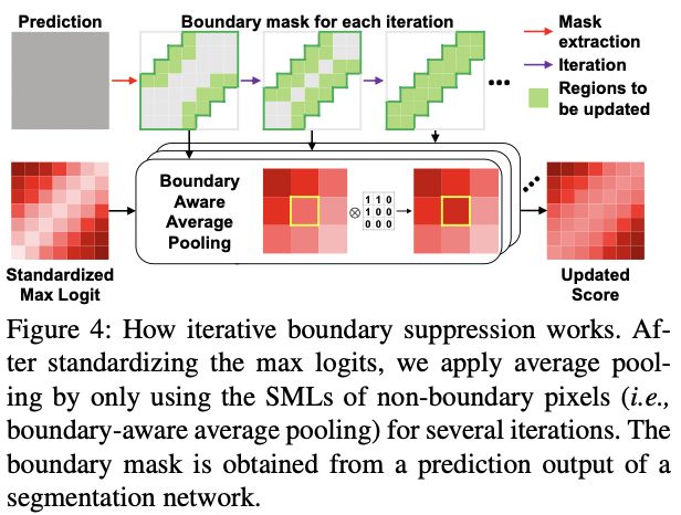
图 4：迭代边界抑制的工作原理。 在标准化最大 logits 之后，我们通过仅使用非边界像素的 SML（即边界感知平均池)进行多次迭代来应用平均池。 边界掩码是从分割网络的预测输出中获得的。

为了解决错误地将边界区域预测为假阳性和假阴性的问题，我们迭代地抑制边界区域。 图 4 说明了迭代边界抑制的过程。 我们逐渐将相邻非边界像素的 SML 传播到边界区域，从边界的外部区域（绿色像素）到内部区域（灰色像素）。 具体来说，我们假设边界宽度为一个特定值，并通过在每次迭代中迭代地减小边界宽度来更新边界。 该过程定义如下。 在第 $i$ 次迭代给定边界宽度 $r_i$ 和语义分割输出 $\hat{Y}$ ，我们得到在每个位置为 $h,w$ 像素的非边界掩码 $M_{h,w}^{(i)}\in {\mathbb{R}}^{H\times W}$ ：
$$M_{h,w}^{(i)}=\{\begin{array}{l}0,if\exists h^{\prime },w^{\prime }s.t.{\hat{Y}}_{h,w}\ne {\hat{Y}}_{h^{\prime },w^{\prime }}\\ 1,otherwise\end{array}\text{\hspace{1em}(6)}$$
for $\forall h^{\prime },w^{\prime }$ that satisfies $|h-h^{\prime }|+|w-w^{\prime }|\le r_i$

Next, we apply the boundary-aware average pooling on the boundary pixels as shown in Fig. 4. This applies average pooling on a boundary pixel only with the SMLs of neighboring non-boundary pixels. With the boundary pixel $b$ and its receptive field $\mathcal{R}$, the boundary-aware average pooling (BAP) is defined as

where $S_{\mathcal{R}}^{(i)}$ and $M_{\mathcal{R}}^{(i)}$ denote the patch of receptive field $\mathcal{R}$ on $S_{\mathcal{R}}^{(i)}$ and $M_{\mathcal{R}}^{(i)}$ , and $(h,w)\in \mathcal{R}$ enumerates the pixels in $\mathcal{R}$. Then, we replace the original value at the boundary pixel $b$ using the newly obtained one. We iteratively apply this process for $n$ times by reducing the boundary width by $\Delta r=2$ at each iteration. We also set the size of receptive field $\mathcal{R}$ as $3\times 3$. In addition, we empirically set the number of iterations n and initial boundary width $r_0$ as 4 and 8.

接下来，我们在边界像素上应用边界感知平均池化，如图 4 所示。这仅在边界像素上应用平均池化，并使用相邻非边界像素的 SML。 使用边界像素 $b$ 及其感受野 $\mathcal{R}$，边界感知平均池化 (BAP) 定义为
$$BAP(S_{\mathcal{R}}^{(i)},M_{\mathcal{R}}^{(i)})=\frac{{\sum }_{h,w}{S}_{\mathcal{R}}^{(i)}\times M_{\mathcal{R}}^{(i)}}{{\sum }_{h,w}{M}_{\mathcal{R}}^{(i)}}\text{\hspace{1em}(7)}$$

$S_{\mathcal{R}}^{(i)}$ 和 $M_{\mathcal{R}}^{(i)}$ 表示 $S_{\mathcal{R}}^{(i)}$ 和 $M_{\mathcal{R}}^{(i)}$ 上的感受野 $\mathcal{R}$ 的补丁 和 $(h,w)\in \mathcal{R}$ 枚举 $\mathcal{R}$ 中的像素。 然后，我们使用新获得的值替换边界像素 $b$ 处的原始值。 我们通过在每次迭代中将边界宽度减小 $\Delta r=2$ 来迭代地应用这个过程 $n$ 次。 我们还将感受野 $\mathcal{R}$ 的大小设置为 $3\times 3$。 此外，我们根据经验将迭代次数 n 和初始边界宽度 $r_0$ 设置为 4 和 8。

3.3.2 Dilated smoothing 扩张平滑

Since iterative boundary suppression only updates boundary pixels, the irregulars in the non-boundary regions are not addressed. Hence, we address these pixels by smoothing them using the neighboring pixels based on the intuition that the local consistency exists among the pixels in a local region. In addition, if the adjacent pixels used for iterative boundary suppression do not have sufficiently low or high anomaly scores, there may still exist boundary pixels that remain as false positives or false negatives even after the process. In this regard, we broaden the receptive fields of the smoothing filter using dilation [41] to reflect the anomaly scores beyond boundary regions.

由于迭代边界抑制只更新边界像素，非边界区域中的不规则不被处理。 因此，我们基于局部区域中像素之间存在局部一致性的直觉，通过使用相邻像素对它们进行平滑来处理这些像素。 此外，如果用于迭代边界抑制的相邻像素没有足够低或足够高的异常分数，则即使在处理之后仍可能存在边界像素保持为假阳性或假阴性。 在这方面，我们使用膨胀 [41] 扩大了平滑滤波器的感受野，以反映边界区域之外的异常分数。

什么是非边界区域中的不规则？

会不会处理了小的异常？会，已经在结论部分给出解释，是不足之处。

For the smoothing filter, we leverage the Gaussian kernel since it is widely known that the Gaussian kernel removes noises [13]. With a given standard deviation σ and convolution filter size k, the kernel weight $K\in {\mathbb{R}}^{k\times k}$ at location $i,j$ is defined as

对于平滑滤波器，我们利用高斯核，因为众所周知，高斯核可以去除噪声 [13]。 在给定标准偏差 σ 和卷积滤波器大小 k 的情况下，位置 $i,j$ 处的核权重 $K\in {\mathbb{R}}^{k\times k}$ 定义为
$$K_{i,j}=\frac{1}{2\pi {\sigma }^2}exp(-\frac{\Delta i^2+\Delta j^2}{2{\sigma }^2})\text{\hspace{1em}(8)}$$
where $∆i=i-(k-1)$ and $∆j=j-(k-1)$ are the displacements of location $i,j$ from the center. In our setting, we set the kernel size $k$ and $\sigma$ to 7 and 1, respectively. Moreover, we empirically set the dilation rate as 6.

其中 $\Delta i=i-(k-1)$ 和 $\Delta j=j-(k-1)$ 是位置 $i,j$ 从中心的位移。 在我们的设置中，我们将内核大小 $k$ 和 $\sigma$ 分别设置为 7 和 1。 此外，我们根据经验将膨胀率设置为 6。

4. Experiments

This section describes the datasets, experimental setup, and quantitative and qualitative results.

本节介绍数据集、实验设置以及定量和定性结果。

4.1. Datasets

Fishyscapes Lost & Found [3] is a high-quality image dataset containing real obstacles on the road. This dataset is based on the original Lost & Found [35] dataset. The original Lost & Found is collected with the same setup as Cityscapes [10], which is a widely used dataset in urban- scene segmentation. It contains real urban images with 37 types of unexpected road obstacles and 13 different street scenarios (e.g., different road surface appearances, strong illumination changes, and etc). Fishyscapes Lost & Found further provides the pixel-wise annotations for 1) unexpected objects, 2) objects with pre-defined classes of Cityscapes [10], and 3) void (i.e., objects neither in pre-defined classes nor unexpected objects) regions. This dataset includes a public validation set of 100 images and a hidden test set of 275 images for the benchmarking

Fishyscapes Lost & Found [3] 是一个高质量的图像数据集，其中包含道路上的真实障碍物。 该数据集基于原始的 Lost & Found [35] 数据集。 原始 Lost & Found 的收集设置与 Cityscapes [10] 相同，Cityscapes [10] 是城市场景分割中广泛使用的数据集。 它包含真实的城市图像，包含 37 种意外道路障碍和 13 种不同的街道场景（例如不同的路面外观、强烈的光照变化等）

Fishyscapes Lost & Found 进一步为 1) 意外对象、2) 具有预先定义的 Cityscapes [10] 类的对象和 3) void（既不在预定义类中也不在意外对象中的对象提供了像素级注释 ) 地区。 该数据集包括 100 张图像的公共验证集和 275 张图像的隐藏测试集，用于基准测试

Fishyscapes Static [3] is constructed based on the validation set of Cityscapes [10]. Regarding the objects in the PASCAL VOC [11] as unexpected objects, they are overlaid on the Cityscapes validation images by using various blending techniques to match the characteristics of Cityscapes. This dataset contains 30 publicly available validation samples and 1,000 test images that are hidden for benchmarking.

Fishyscapes Static [3] 是基于 Cityscapes [10] 的验证集构建的。 将 PASCAL VOC [11] 中的对象视为意外对象，通过使用各种混合技术将它们叠加在 Cityscapes 验证图像上以匹配 Cityscapes 的特征。 该数据集包含 30 个公开可用的验证样本和 1,000 个隐藏用于基准测试的测试图像。

Road Anomaly [26] contains images of unusual dangers which vehicles confront on roads. It consists of 60 web-collected images with anomalous objects ( animals, rocks, and etc.) on roads with a resolution of 1280 × 720. This dataset is challenging since it contains various driving circumstances such as diverse scales of anomalous objects and adverse road conditions.

Road Anomaly [26] 包含车辆在道路上遇到的异常危险的图像。 它由 60 个网络收集的图像组成，在道路上具有异常物体（动物、岩石等），分辨率为 1280 × 720。该数据集具有挑战性，因为它包含各种驾驶环境，例如不同尺度的异常物体和不利的道路条件。

4.2 Experimental Setup

Implementation Details We adopt DeepLabv3+ [7] with ResNet101 [15] backbone for our segmentation architecture with the output stride set to 8. We train our segmentation networks on Cityscapes [10] which is one of the widely used datasets for urban-scene segmentation. We use the same pre-trained network for all experiments.

Evaluation Metrics For the quantitative results, we compare the performance by the area under receiver operating characteristics (AUROC) and average precision (AP). In addition, we measure the false positive rate at a true positive rate of 95% (FPR95) since the rate of false positives in high-recall areas is crucial for safety-critical applications. For the qualitative analysis, we visualize the prediction results using the threshold at a true positive rate of 95% (TPR95).

Baselines We compare ours with the various approaches reported in the Fishyscapes leaderboard. We also report results on the Fishyscapes validation sets and Road Anomaly with previous approaches that do not utilize external datasets or require additional training for fair comparisons. Additionally, we compare our method with approaches that are not reported in the Fishyscapes leaderboard. Thus, we include the previous method using max logit [16] and SynthCP [39] that leverages an image resynthesis model for such comparison. Note that SynthCP requires training of additional networks.

实现细节 我们采用 DeepLabv3+ [7] 和 ResNet101 [15] 主干作为我们的分割架构，输出步幅设置为 8。我们在 Cityscapes [10] 上训练我们的分割网络，这是广泛使用的城市数据集之一 -场景分割。 我们对所有实验使用相同的预训练网络。

评估指标 对于定量结果，我们按接收器操作特性 (AUROC) 和平均精度 (AP) 下的区域比较性能。 此外，我们以 95% 的真阳性率 (FPR95) 测量误报率，因为高召回率区域的误报率对于安全关键型应用至关重要。 对于定性分析，我们使用阈值以 95% 的真阳性率 (TPR95) 可视化预测结果。

基线 我们将我们的方法与 Fishyscapes 排行榜中报告的各种方法进行比较。 我们还报告了 Fishyscapes 验证集和 Road Anomaly 的结果，这些方法不使用外部数据集或需要额外培训以进行公平比较。 此外，我们将我们的方法与 Fishyscapes 排行榜中未报告的方法进行比较。 因此，我们使用了之前使用最大 logit [16] 和 SynthCP [39] 的方法，该方法利用图像再合成模型进行此类比较。 请注意，SynthCP 需要训练额外的网络。

4.3 Evaluation Results

This section provides the quantitative and qualitative re- sults. We first show the results on Fishyscapes datasets and Road Anomaly, and then present the comparison results with various backbone networks. Additionally, we report the computational cost and the qualitative results by com- paring with previous approaches.

本节提供定量和定性结果。 我们首先展示了 Fishyscapes 数据集和 Road Anomaly 的结果，然后展示了与各种骨干网络的比较结果。 此外，我们通过与以前的方法进行比较来报告计算成本和定性结果。

4.3.1 Comparison on Fishyscapes Leaderboard 排行榜比较

Table 1 shows the leaderboard result on the test sets of Fishyscapes Lost & Found and Fishyscapes Static. The Fishyscapes Leaderboard categorizes approaches by check- ing whether they require retraining of segmentation net- works or utilize OoD data. In this work, we add the Ex- tra Network column under the Additional Training category. Extra networks refer to the extra learnable parameters that need to be trained using a particular objective function other than the one for the main segmentation task. Utilizing extra networks may require a lengthy inference time, which could be critical for real-time applications such as autonomous driving. Considering such importance, we add this category for the evaluation.

As shown in Table 1, we achieve a new state-of-the-art performance on the Fishyscapes Lost & Found dataset with a large margin, compared to the previous models that do not require additional training of the segmentation network and external datasets. Additionally, we even outperform 6 previous approaches in Fishyscapes Lost & Found and 5 models in Fishyscapes Static which fall into at least one of the two categories. Moreover, as discussed in the previous work [3], retraining the segmentation network with addi- tional loss terms impair the original segmentation perfor- mance(i.e., mIoU) as can be shown in the cases of Bayesian Deeplab [31], Dirichlet Deeplab [29], and OoD Training with void class in Table 1. This result is publicly available on the Fishyscapes benchmark website.

表 1 显示了 Fishyscapes Lost & Found 和 Fishyscapes Static 测试集的排行榜结果。 Fishyscapes 排行榜通过检查它们是否需要重新训练分割网络或利用 OoD 数据来对方法进行分类。 在这项工作中，我们在 Additional Training 类别下添加了 Extra Network 列。 额外网络是指需要使用特定目标函数训练的额外可学习参数，而不是用于主要分割任务的目标函数。 利用额外的网络可能需要很长的推理时间，这对于自动驾驶等实时应用至关重要。 考虑到这样的重要性，我们添加了这个类别进行评估。

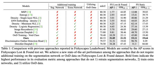
表 1：与 Fishyscapes 排行榜中报告的先前方法的比较。 模型按 Fishyscapes Lost & Found 测试集中的 AP 分数排序。 我们在不需要对分割网络或 Fishyscapes Lost & Found 数据集的 OoD 数据进行额外训练的方法中实现了新的最先进的性能。 粗体表示其评估指标在方法网络中的最高性能，并且 3)利用 OoD 数据。

如表 1 所示，与不需要对分割网络和外部数据集进行额外训练的先前模型相比，我们在 Fishyscapes Lost & Found 数据集上实现了新的最先进的性能。 此外，我们甚至超过了 Fishyscapes Lost & Found 中的 6 个先前方法和 Fishyscapes Static 中的 5 个模型，它们至少属于这两个类别中的一个。 此外，正如在之前的工作 [3] 中所讨论的，使用额外的损失项重新训练分割网络会损害原始分割性能（即 mIoU），这可以在贝叶斯 Deeplab [31]、Dirichlet Deeplab 的案例中得到证明 [29]，以及表 1 中带有 void 类的 OoD 训练。该结果可在 Fishyscapes 基准网站上公开获得。

4.3.2 Comparison on Fishyscapes validation sets and Road Anomaly

For a fair comparison, we compare our method on Fishyscapes validation sets and Road Anomaly with pre- vious approaches which do not require additional training and OoD data. As shown in Table 2, our method outper- forms other previous methods in the three datasets with a large margin. Additionally, our method achieves a signifi- cantly lower FPR95 compared to previous approaches.

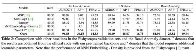
表 2：与 Fishyscapes 验证集和 Road Anomaly 数据集中其他基线的比较。 † 表示结果是使用我们预先训练的主干从官方代码中获得的，∗ 表示该模型需要额外的可学习参数。 请注意，kNN Embedding - Density 的性能由 Fishyscapes [3] 团队提供。

为了公平比较，我们将 Fishyscapes 验证集和 Road Anomaly 的方法与之前不需要额外训练和 OoD 数据的方法进行比较。 如表 2 所示，我们的方法在三个数据集中以较大的优势优于其他先前的方法。 此外，与以前的方法相比，我们的方法实现了显着降低的 FPR95。

4.3.3 Qualitative Analysis

Fig. 5 visualizes the pixels detected as unexpected objects (i.e., white regions) with the TPR at 95%. While previous approaches using MSP [18] and max logit [16] require nu- merous in-distribution pixels to be detected as unexpected, our method does not. To be more specific, regions that are less confident (e.g., boundary pixels) are detected as un- expected in MSP [18] and max logit [16]. However, our method clearly reduces such false positives which can be confirmed by the significantly reduced number of white regions.

图 5：使用 TPR95 检测到的意外对象。 我们将我们的方法与 MSP [18] 和 max logit [16] 进行比较。 白色像素表示被识别为意外对象的对象。 与这两种方法相比，我们的方法显着减少了误报像素的数量。

图 5 将检测到的像素可视化为意外物体（即白色区域），TPR 为 95%。 虽然以前使用 MSP [18] 和 max logit [16] 的方法需要将大量分布内像素检测为意外，但我们的方法不需要。 更具体地说，在 MSP [18] 和最大 logit [16] 中检测到的置信度较低的区域（例如边界像素)是出乎意料的。 然而，我们的方法明显减少了这种误报，这可以通过显着减少的白色区域数量来证实。

5.Discussion

In this section, we conduct an in-depth analysis on the effects of our proposed method along with the ablation studies.

在本节中，我们对我们提出的方法以及消融研究的效果进行了深入分析。

5.1. Ablation Study

Table 3 describes the effect of each proposed method in our work with the Fishyscapes Lost & Found validation set. SML achieves a significant performance gain over using the max logit [16]. Performing iterative boundary suppression on SMLs improves the overall performance (i.e., 4% increase in AP and 1% decrease in FPR95). On the other hand, despite the increase in AP, performing dilated smoothing on SMLs without iterative boundary suppression results in an unwanted slight increase in FPR95. The following is the possible reason for the result. When dilated smoothing is applied without iterative boundary suppression, the anomaly scores of non-boundary pixels may be updated with those of boundary pixels. Since the non-boundary pixels of in-distribution objects have low anomaly scores compared to the boundaries, it may increase false positives. Such an issue is addressed by performing iterative boundary suppression before applying dilated smoothing. After the boundary regions are updated with neighboring non-boundary regions, dilated smoothing increases the overall performance without such error propagation.

表 3 描述了在我们使用 Fishyscapes Lost & Found 验证集的工作中每种建议方法的效果。 与使用最大 logit [16] 相比，SML 获得了显着的性能提升。 对 SML 执行迭代边界抑制可提高整体性能（即 AP 增加 4%，FPR95 减少 1%）。 另一方面，尽管 AP 增加，但在没有迭代边界抑制的情况下对 SML 执行扩张平滑会导致 FPR95 略有增加。 以下是该结果的可能原因。 当在没有迭代边界抑制的情况下应用扩张平滑时，非边界像素的异常分数可能会随着边界像素的异常分数而更新。 由于分布对象的非边界像素与边界相比具有较低的异常分数，因此可能会增加误报。 通过在应用扩张平滑之前执行迭代边界抑制来解决此类问题。 在使用相邻的非边界区域更新边界区域后，扩张平滑提高了整体性能，而不会出现这种错误传播。

5.2 Analysis

This section provides an indepth analysis on the effects on segmentation performance, comparison with various backbones, and comparison on computational costs.

本节深入分析了对分割性能的影响，与各种骨干网的比较，以及计算成本的比较。

5.2.1 Effects on the segmentation performance

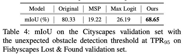
Table 4 shows the mIoU on the Cityscapes validation set with the detection threshold at TPR95. By applying the detection threshold, the segmentation model predicts a nontrivial amount of in-distribution pixels as the unexpected ones. Due to such false positives, the mIoU of all meth- ods decreased from the original mIoU of 80.33%. To be more specific, using MSP [18] and max logit [16] result in significant performance degradation. On the other hand, our approach maintains a reasonable performance of mIoU even with outstanding unexpected obstacle detection perfor- mance. This table again demonstrates the practicality of our work since it both shows reasonable performance in the seg- mentation task and the unexpected obstacle detection task.

通过mIoU发现：概率置信度预测的方法容易出现假阳性。并展现了本文方法的有效性

表4显示了检测阈值为TPR95的城市景观验证集上的mIoU。通过应用检测阈值，分割模型将大量的分布内像素预测为意外的像素。由于这种假阳性，所有方法的mIoU从原来的80.33%下降。更具体地说，使用MSP[18]和max logit[16]会导致性能显著下降。另一方面，我们的方法保持了合理的mIoU的性能，甚至有突出的意外障碍物检测性能。这个表格再次证明了我们工作的实用性，因为它同时显示了在隔离任务和意外障碍物检测任务中的合理性能。

5.2.2 Comparison with various backbones

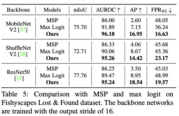
Since our method does not require additional training or extra OoD datasets, our method can be adopted and used easily on any existing pretrained segmentation networks. To verify the wide applicability of our approach, we report the performance of identifying anomalous objects with various backbone networks including MobileNetV2 [37], ShuffleNetV2 [28], and ResNet50 [28]. As shown in Table 5, our method significantly outperforms the other approaches [18, 16] using the same backbone network with a large improvement in AP. This result clearly demonstrates that our method is applicable widely regardless of the backbone network.

由于我们的方法不需要额外的训练或额外的OoD数据集，我们的方法可以很容易地在任何现有的预训练的分割网络上采用和使用。为了验证我们方法的广泛适用性，我们报告了用各种骨干网络识别异常对象的性能，包括MobileNetV2[37]、ShuffleNetV2[28]和ResNet50[28]。如表5所示，我们的方法在使用相同的骨干网络时明显优于其他方法[18, 16]，在AP方面有很大的改进。这一结果清楚地表明，无论骨干网络如何，我们的方法都能广泛适用。

5.2.3 Comparison on computational cost

To demonstrate that our method requires a negligible amount of computation cost, we report GFLOPs (i.e., the number of floating-point operations used for computation) and the inference time. As shown in Table 6, our method requires only a minimal amount of computation cost regarding both GFLOPs and the inference time compared to the original segmentation network, ResNet-101 [15]. Also, among several studies which utilize additional networks, we compare with a recently proposed approach [39] that leverages an image resynthesis model. Our approach requires substantially less amount of computation cost compared to SynthCP [39].

为了证明我们的方法需要的计算成本可以忽略不计，我们报告了GFLOPs（即用于计算的浮点运算次数）和推理时间。如表6所示，与原始分割网络ResNet-101[15]相比，我们的方法在GFLOPs和推理时间方面都只需要极少的计算成本。另外，在一些利用额外网络的研究中，我们与最近提出的利用图像再合成模型的方法[39]进行比较。与SynthCP[39]相比，我们的方法需要的计算成本大大减少。

5.3. Effects of Standardized Max Logit

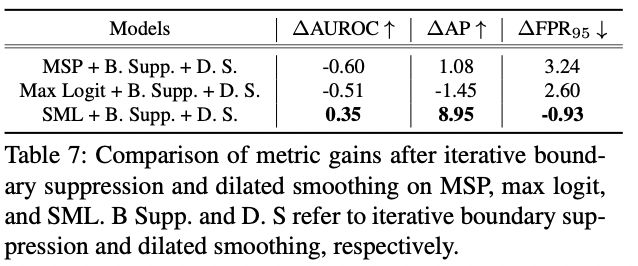
Table 7 describes how SML enables applying iterative boundary suppression and dilated smoothing. Applying iterative boundary suppression and dilated smoothing on other approaches does not improve the performance or even aggravates in the cases of MSP [18] and max logit [16]. On the other hand, it significantly enhances the performance when applied to SML. The following are the possible reasons for such observation. As aforementioned, the overconfidence of the softmax layer elevates the MSPs of anomalous objects. Since the MSPs of anomalous objects and in-distribution objects are not distinguishable enough, applying iterative boundary suppression and dilated smoothing may not improve the performance.

表7描述了SML如何实现迭代边界抑制和扩张平滑的应用。在其他方法上应用迭代边界抑制和扩张平滑并不能提高性能，甚至在MSP[18]和max logit[16]的情况下会恶化。另一方面，当应用于SML时，它明显提高了性能。以下是这种观察的可能原因。如前所述，softmax层的过度自信提高了异常对象的MSP。由于异常对象的MSP和分布中的对象没有足够的区别，应用迭代边界抑制和扩张平滑可能不会提高性能。

Additionally, iterative boundary suppression and dilated smoothing require the values to be scaled since it performs certain computations with the values. In the case of using max logits, the values of each predicted class differ accord- ing to the predicted class. Performing the iterative bound- ary suppression and dilated smoothing in such a case aggra- vates the performance because the same max logit values in different classes represent different meanings according to their predicted class. SML aligns the differently formed dis- tributions of max logits which enables to utilize the values of neighboring pixels with certain computations.

此外，迭代边界抑制和扩张平滑需要对数值进行缩放，因为它对数值进行了某些计算。在使用最大对数的情况下，每个预测类的值根据预测类的不同而不同。在这种情况下，执行迭代边界抑制和扩张平滑会提高性能，因为不同类别中相同的最大对数值根据其预测类别代表不同的意义。SML对不同的最大对数分布进行了调整，这使得在某些计算中可以利用邻近像素的值。

6. Conclusions

In this work, we proposed a simple yet effective method for identifying unexpected obstacles on roads that do not require external datasets or additional training. Since max logits have their own ranges in each predicted class, we aligned them via standardization, which improves the performance of detecting anomalous objects. Additionally, based on the intuition that pixels in a local region share local semantics, we iteratively suppressed the boundary regions and re- moved irregular pixels that have distinct values compared to neighboring pixels via dilated smoothing. With such a straightforward approach, we achieved a new state-of-the-art performance on Fishyscapes Lost & Found benchmark. Additionally, extensive experiments with diverse datasets demonstrate the superiority of our method to other previous approaches. Through the visualizations and in-depth analysis, we verified our intuition and rationale that standardizing max logit and considering the local semantics of neighbor- ing pixels indeed enhance the performance of identifying unexpected obstacles on roads. However, there still remains room for improvements; 1) dilated smoothing might remove unexpected obstacles that are as small as noises, and 2) the performance depends on the distribution of max logits ob- tained from the main segmentation networks.

在这项工作中，我们提出了一个简单而有效的方法来识别道路上的意外障碍物，该方法不需要重新引用外部数据集或额外的训练。由于最大对数在每个预测类中都有自己的范围，我们通过标准化将其对齐，这提高了检测异常物体的性能。此外，基于局部区域的像素共享局部语义的直觉，我们迭代地抑制了边界区域，并通过扩张平滑重新移动了与相邻像素相比具有明显价值的不规则像素。通过这种直接的方法，我们在Fishyscapes Lost & Found基准测试中取得了最先进的性能。此外，在不同的数据集上进行的广泛实验证明了我们的方法比以前的其他方法更有优势。通过可视化和深入分析，我们验证了我们的直觉和理由，即标准化的最大对数和考虑相邻像素的局部语义确实提高了识别道路上意外障碍物的性能。然而，仍有改进的余地；1）扩张平滑可能会去除像噪音一样小的意外障碍物；2）性能取决于从主要分割网络中获得的最大对数的分布。

We hope our work inspires the following researchers to investigate such practical methods for identifying anomalous objects in urban-scene segmentation which is crucial in safety-critical applications.

我们希望我们的工作能激励以下研究人员研究这种实用的方法，以识别城市场景分割中的异常物体，这对安全关键应用至关重要。

---

1. Robustnet: Improving domain generalization in urban-scene segmentation via instance selective whitening. ↩︎

2. Cars can’t fly up in the sky: Improving urban-scene segmentation via height-driven attention networks. ↩︎

3. Foveanet: Perspective-aware urban scene parsing. ↩︎

4. Denseaspp for semantic segmentation in street scenes. ↩︎

5. Improving semantic segmentation via video propagation and label relaxation ↩︎

6. Asymmetric non-local neural networks for semantic segmentation ↩︎

7. Dual attention network for scene segmentation ↩︎